Design, simulation, and fabrication of a flow sensor for an implantable micropump

Rochester Institute of Technology

RIT Scholar Works

Theses Thesis/Dissertation Collections

12-1-2009

Design, simulation, and fabrication of a flow sensor

for an implantable micropump

Matthew J. Waldron

Follow this and additional works at:http://scholarworks.rit.edu/theses

This Thesis is brought to you for free and open access by the Thesis/Dissertation Collections at RIT Scholar Works. It has been accepted for inclusion in Theses by an authorized administrator of RIT Scholar Works. For more information, please [email protected].

Recommended Citation

Design, Simulation, and Fabrication of a Flow Sensor

for an Implantable Micropump

by

Matthew J. Waldron

A Graduate Thesis Submitted in Partial Fulfillment

of the Requirements for the Degree of

MASTER OF SCIENCE

in

Electrical Engineering

Approved by:

Dr. David Borkholder, Thesis Advisor

Dr. James Moon, Committee Member

Dr. Lynn Fuller, Committee Member

Dr. Sohail Dianat, Department Head

DEPARTMENT OF ELECTRICAL AND MICROELECTRONIC ENGINEERING KATE GLEASON COLLEGE OF ENGINEERING

A

The design, simulation, and fabrication of a flow sensor to be integrated into an implantable micropump is presented. The flow sensor operates by the method of thermal anemometry, in which heat is dissipated from a resistive element held in the flow of the fluid. The rate at which heat is carried away is dependent on the flow rate and is directly related to the thermal conductance. A control circuit utilizing the constant-temperature anemometry mode of operation is used to generate a change in voltage in response to change in thermal conductance, and subsequently, flow rate.

A mathematical expression describing the sensor sensitivity based on thermal effects is proposed, based on the thermal spreading resistance and basic heat transfer laws. The mathematical model is refined using finite-element analysis, and a complete formulation for the effect of sensor area, length-to-width ratio, and fluid velocity on thermal spreading resistance is determined. The refined thermal spreading conductance equation can be used to replace assumptions made in initial mathematical analysis.

An original fabrication process is presented and investigated, in which a p-doped polysilicon bridge is encapsulated in silicon oxide and silicon nitride using surface micromachining techniques. A sacrificial polysilicon layer and KOH etching are used to form half of the complete fluid channel in the bulk of the silicon wafer. When the fluid channel is sealed with a complementarily etched wafer, the sensor bridge is situated in the middle of the fluid channel, optimally placed for maximum sensitivity. The fabrication process yields functional sensor bridges, with even the most fragile sensor shape withstanding the process.

T

C

List of Tables ... ii

List of Figures ... iii

Chapter 1: Background ...1

Chapter 2: Thermal Flow Measurement ...9

I. Modes of Operation ...10

II. Sensor Design ...13

Chapter 3: Physics of Operation ...19

I. Electrical Domain ...21

II. Thermal Domain ...23

III. MATLAB Analysis...32

Chapter 4: Finite-Element Analysis...43

I. Simulation Setup...44

II. Thermal Spreading Conductance ...47

III. Simulation of Entire System ...71

Chapter 5: Fabrication...83

I. Fabrication Procedure and Process Details...84

II. Fabrication Yield ...109

Chapter 6: Signal-Conditioning Circuitry...121

Chapter 7: Test Plan...145

I. Fluid Channel Formation ...145

II. Thermal Characterization...148

Chapter 8: Coalescence of Results...152

I. Overall Sensitivity Prediction...153

II. Future Work...156

Appendix A: MATLAB Scripts for Chapter 3 ...158

Appendix B: MATLAB Scripts for Chapter 4...162

Appendix C: CGS Units...174

L

T

Table 3.1: Sensor Geometry Parameters... 20

Table 3.2: Thermal Domain Parameters ... 25

Table 3.3: Fluid Property Variables... 29

Table 3.4: Nominal Sensor Parameters in MATLAB Simulations... 32

Table 4.1: Values of the Coefficients of the Quartic Function fitted to Simulation Data of Thermal Spreading Conductance... 58

Table 4.2: Values of the Coefficients of the Quartic Function with Additional Parameter for Area Dependence... 60

Table 4.3: Fitting Parameters for King’s Law Coefficient ... 65

Table 4.4: Results of Simulation with 32 µm Fluid Channel ... 77

Table 4.5: Results of Simulation with 60 µm Fluid Channel ... 79

Table 4.6: Results of Simulation with 100 µm Fluid Channel ... 80

Table 8.1 Sensitivities for Simulated Circuits in Chapter 6... 154

Table 8.2 Typical and Minimum Overall Sensitivities for Circuits in Chapter 6... 154

L

F

Figure 1.1: Turbine flowmeter diagram... 2

Figure 1.2: Oval gear positive displacement flowmeter. ... 3

Figure 1.3: Orifice plate in a fluid channel with pressure taps. ... 4

Figure 1.4: Example of a microscale differential pressure sensor... 4

Figure 1.5: Example of an electromagnetic flow sensor... 5

Figure 2.1: Basic hot-wire anemometer diagram... 9

Figure 2.2: Calorimeter type flow sensor. ... 10

Figure 2.3: Heat pulses observed from a thermal time-of-flight sensor. ... 11

Figure 2.4: Example of a thermal anemometer in a fluid channel made from a silicon wafer and glass wafer. ... 16

Figure 3.1: Thermal anemometer diagram for electrical and thermal analysis. ... 19

Figure 3.2: Diagram of geometric variables. ... 20

Figure 3.3: Electrical domain diagram. ... 21

Figure 3.4: Electrical characteristics vs. distance from channel wall for typical anemometer geometry. ... 22

Figure 3.5: Diagram of heat conduction. ... 23

Figure 3.6: Thermal equivalent circuit diagram. ... 26

Figure 3.7: Thermal spreading resistance vs. length-to-width ratio with best-fit curves. ... 27

Figure 3.8: Spreading resistance vs. logarithm of the length-to-width ratio. ... 28

Figure 3.9: Thermal conductance vs. flow rate... 33

Figure 3.10: Anemometer power dissipation vs. flow rate... 34

Figure 3.11: Anemometer voltage vs. flow rate. ... 34

Figure 3.12: Thermal conductance vs. length-to-width ratio with constant area... 36

Figure 3.13: Thermal conductance vs. heater area with length-to-width ratio held constant... 37

Figure 3.14: Thermal conductance vs. heater width... 38

Figure 3.15: Thermal conductance vs. channel width. ... 39

Figure 3.16: Sensitivity vs. channel width... 40

Figure 4.1: ANSYS model of an anemometer in fluid channel... 44

Figure 4.5: Meshed rectangular prisms using finest smart sizing resolution... 49

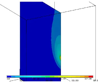
Figure 4.6: Contour plot of temperature with fluid velocity fixed at zero... 50

Figure 4.7: Vector plot of fluid velocity with maximum fluid velocity. ... 51

Figure 4.8: Contour plot of temperature with maximum fluid velocity across the sensor. ... 52

Figure 4.9: Contour plot of temperature along the direction of fluid flow... 52

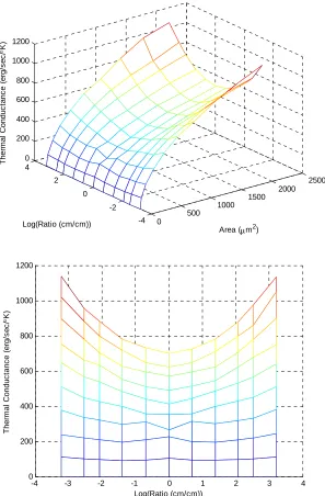
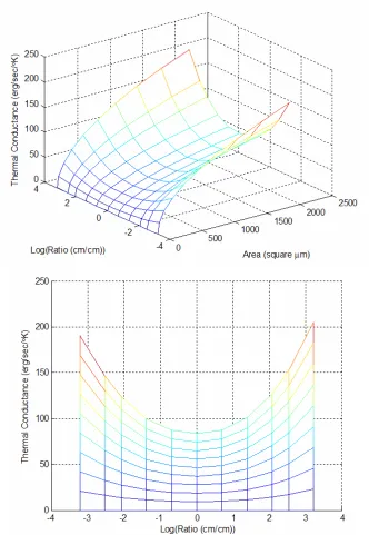
Figure 4.10: Surface plot of thermal conductance versus length-to-width ratio and area at zero flow rate... 54

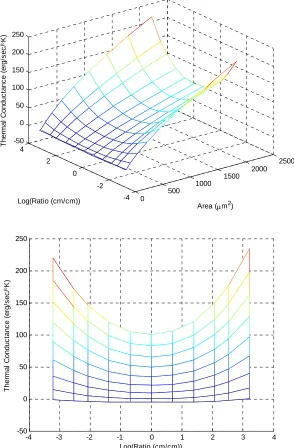
Figure 4.11: Surface plot of thermal conductance versus length-to-width ratio and area at 0.3 cm/sec. ... 55

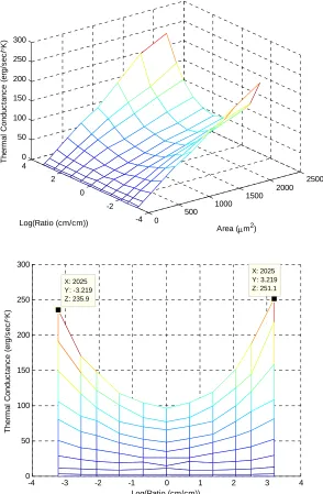
Figure 4.12: Surface plot of the difference in thermal conductance at 0.3 cm/sec and zero flow versus length-to-width ratio and area. ... 56

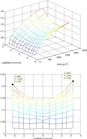
Figure 4.13: Surface plot of the ratio of thermal conductance at 0.3 cm/sec to zero flow versus length-to-width ratio and area... 57

Figure 4.14: Surface plot of the difference in thermal conductance at flow rate of 0.3 cm/sec and zero flow rate, calculated from fitted quartic function for thermal spreading conductance... 59

Figure 4.15: Surface plot of the difference in thermal conductance at flow rates of 0.3 cm/sec and 0, calculated from the fitted quartic function with area dependence for thermal spreading conductance. ... 61

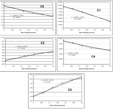
Figure 4.16: Plot of curve fitting coefficients, C0, C1, C2, C4, and C5 versus flow velocity with linear trendlines. ... 62

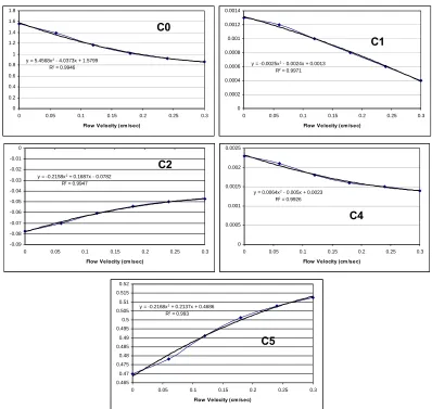
Figure 4.17: Plot of curve fitting coefficients, C0, C1, C2, C4, and C5 versus flow velocity with second-order polynomial trendlines. ... 63

Figure 4.18: King’s Law coefficient, β, versus sensor area and length-to-width ratio fitted to the simulation data for thermal conductance... 64

Figure 4.19: King’s Law exponent, χ, versus sensor area and length-to-width ratio fitted to the simulation data for thermal conductance... 65

Figure 4.20: Relative sensitivity to fluid velocity at 0.15 cm/sec versus sensor area and thermal length to width ratio calculated using quartic fit of thermal conductance data. ... 68

Figure 4.21: Relative sensitivity to fluid velocity at 0.15 cm/sec versus sensor area and thermal length to width ratio calculated using the King’s Law fit of thermal conductance data. ... 68

Figure 4.22: Sensor quality factor at 0.15 cm/sec versus sensor area and thermal length to width ratio calculated using the quartic fit of thermal conductance data. ... 70

Figure 4.23: Sensor quality factor at 0.15 cm/sec versus sensor area and thermal length to width ratio calculated using the King’s Law fit of thermal conductance data. ... 70

Figure 4.24: Results of velocity magnitude component parallel to microchannel. ... 73

Figure 4.27: Total thermal conductance vs. flow rate for ANSYS simulations. ... 75

Figure 4.28: Velocity dependent thermal conductance vs. flow rate... 76

Figure 4.29: Velocity dependent thermal conductance for sensors in a 32 µm fluid channel... 78

Figure 4.30: Velocity dependent thermal conductance for sensors in a 60 µm fluid channel... 80

Figure 4.31: Velocity dependent thermal conductance for sensors in a 100 µm fluid channel... 81

Figure 5.1: Color legend of materials in microfabrication. ... 84

Figure 5.2: Tensile and compressive wafer bending after deposition of silicon nitride... 92

Figure 5.3: Fit of resistivity versus diffusion temperature for Emulsitone spin-on dopants. ... 96

Figure 5.4: CDE ResMap analysis of N250 dopant diffused into polysilicon after second diffusion... 96

Figure 5.5: CDE ResMap analysis of Borofilm 100 dopant diffused into polysilicon after second diffusion... 97

Figure 5.6: Cross-sectional profile of KOH etch on (100) silicon... 108

Figure 5.7: Cross-section of the complete anemometer fabrication process. ... 109

Figure 5.8: Microscope image of fabrication after step 34... 110

Figure 5.9: Microscope image of fabrication after step 34 showing residue inhibiting the phosphoric acid etch. ... 111

Figure 5.10: Microscope image of fabrication after completed fabrication showing residue remaining attached to bridges... 112

Figure 5.11: Microscope image showing typical sensor and fluid channel at difference focus depths... 113

Figure 5.12: Microscope image of sensor after completed fabrication process. ... 114

Figure 5.13: SEM image of 60 µm fluid channel entrance... 115

Figure 5.14: SEM image of 32 µm fluid channel entrance... 115

Figure 5.15: SEM image of typical sensor in 100 µm fluid channel... 116

Figure 5.16: SEM image of wide sensor in 60 µm fluid channel. ... 116

Figure 5.17: SEM image of encapsulated serpentine polysilicon bridge. ... 117

Figure 5.18: SEM image of crease in layers at fluid channel edge. ... 118

Figure 5.19: SEM image of sensor in 60 µm fluid channel to aluminum traces. ... 118

Figure 6.1: Basic Wheatstone bridge with constant bridge voltage... 123

Figure 6.5: Heater circuit element coupling electrical circuit and thermal equivalent circuit... 129

Figure 6.6: Wheatstone bridge with feedback op-amp with thermal properties of the heater resistor (right) and ambient temperature sensor (left) taken considered. ... 130

Figure 6.7: Transient simulation results of the circuit in Figure 6.6. ... 131

Figure 6.8: DC Sweep simulation results of the circuit in Figure 6.6. ... 131

Figure 6.9: Results of varying overheat temperature in Figure 6.6. ... 132

Figure 6.10: Dependence of circuit sensitivity on overheat temperature. ... 133

Figure 6.11: Wheatstone bridge with feedback op-amp and thermal characteristics given to both the heating resistor and ambient temperature sensor... 134

Figure 6.12: Simulation results of circuit in Figure 6.11. The thermal resistance is swept on the x-axis. The upper plot shows the voltage of the op-amp output, and the lower plot shows the overheat temperature of the sensor... 134

Figure 6.13: Effect of changing the value of the ambient temperature sensor in Figure 6.11 on quality factor... 136

Figure 6.14: Wheatstone bridge with feedback amplifier circuit with ambient temperature sensor element replaced with transimpedance circuit... 138

Figure 6.15: Output voltage of the circuit in Figure 6.14 versus thermal resistance... 139

Figure 6.16: Effect of changing amplifier gain of diff amp 2 in the circuit in Figure 6.14 on quality factor... 140

Figure 6.17: Amplifier gain of diff amp 2 in the circuit in Figure 6.14 to produce maximum quality factor... 140

Figure 6.18: Wheatstone bridge with feedback amplifier and ambient side voltage reduction... 141

Figure 6.19: Output voltage of the circuit in Figure 6.18 versus thermal resistance with different ambient temperatures... 142

Figure 6.20: Effect of changing amplifier gain in Figure 6.18 on quality factor... 143

Figure 7.1: Anisotropically etched silicon wafer bonded to isotropically etched glass wafer. ... 146

Figure 7.2: Schematic of complete constant-power characterization circuit... 149

Figure 7.3: Anemometer power from Figure 7.2... 150

B

ACKGROUND

In microscale drug delivery systems, flow measurement performs a critical role in the pump feedback loop. In open-loop micropump systems, the pump behavior is initially characterized, and driven to deliver the amount of fluid desired. If the pump behavior degrades or changes over time, the pump’s ability to dispense a precise amount of fluid worsens. By adding a flow sensor to the pump control system, the system becomes closed-loop, and the pump can compensate for changes in behavior to dispense the desired amount of fluid.

Micropumps, and microfluidics in general, have found a niche in biological and medical applications. Microfluidic assays can be used to assess the results of biological and chemical reactions using very small amounts of reactants. Implantable micropumps can be used to administer drugs over a long period of time, without the need for repeated injections, and breaching of the skin by needles ([6]). In drug-delivery systems, ensuring that the correct dose is administered is crucial, and in research applications when the dosage may need to be varied, the feedback provided by the flow sensor helps to ensure the accuracy of the experiment.

Flow sensors that use the fluid flow to drive mechanical motion are very common in macroscale systems. A turbine is one type of flowmeter that uses this principle, seen in Figure 1.1. Fluid flows in the direction of the red arrows. Bearings and a physical support hold the turbine in place, and the flowing fluid pushes on the turbine blades, causing the turbine to spin. The rotational velocity can be measured, and correlated to the fluid velocity. An apparatus on the outside of the pipe detects when the turbine blades pass to calculate the rotational velocity. If that region of the pipe is transparent, the turbine blades can be detected optically. Magnetic pickups can be used to detect when blades pass by the detector. Similarly, the change in electrical capacitance can also be used to detect spinning blades ([10]).

Figure 1.1: Turbine flowmeter diagram.

Figure 1.2: Oval gear positive displacement flowmeter.

At the macroscale, turbines and positive displacement flow meters are usually the most accurate. The high accuracy of positive displacement flowmeters is evident since they control how much fluid flows through them, and eliminate the effects of turbulence in the flow. This accuracy comes at the expense of a very high pressure drop across the sensor. In the oval gear, and similar positive displacement flowmeters, the fluid must force the gears to turn, acting against inertia and friction, from both the gear bearings and the fluid. In the turbine, drag forces on the turbine blades and bearing friction are the cause for a significant pressure drop. At the microscale, these designs, like most devices with moving parts, are very difficult to create. They require the fabrication of complex geometric structures, such as the blades of the turbine, and would typically need to be assembled by bonding parts made on separate wafers.

Figure 1.3: Orifice plate in a fluid channel with pressure taps.

The hydraulic resistance of the constriction dictates the relationship between the pressure drop and the fluid velocity. This can be determined analytically or empirically, and while it is usually constant, the hydraulic resistance can be very mathematically complicated or variable, depending on the flow turbulence and the geometry of the constriction. Like the positive displacement flowmeter, as the fluid passes through the sensor, a large drop in pressure is incurred. This is undesirable since it adds more load to the pumping system, but is still favorable over positive displacement type flowmeters since no moving parts are required, making the differential pressure sensor much simpler to fabricate for microscale applications. Figure 1.4 shows an example of a differential pressure flow sensor compatible with micromachining processes. Two wafers are bonded together: one wafer with two chambers and a narrow flow channel between the chambers; another wafer that seals the channel and provides inlet and outlet ports to the two chambers. The flow of fluid follows the red arrows at the inlet and outlet. The micromachined fluid channel provides the constriction, and the pressure in the two cavities, PIN and POUT,

the membrane deflection and determine the difference in pressure in the two chambers ([4], [5], [9]).

In battery-powered microfluidic systems, where low voltage and limited energy are used to drive the pump, the performance can be significantly abated by pumping against a large hydraulic resistance. To avoid such drops in pressure, the use of a sensor that can be integrated into the fluid channel without constriction is essential. Still, many sensor types exist with this attribute. If the fluid is charged, then a sensor utilizing the Lorentz force can be created. In the presence of a magnetic field, charged molecules in the fluid flow experience a force, which can be measured as an electrical voltage, demonstrated in Figure 1.5. Fluid flows in the direction of the red arrows, and the coils on either side of the fluid channel produce a magnetic field in the direction of the green arrows. A voltage proportional to the fluid velocity and magnetic field strength will be detected on electrodes placed perpendicular to the direction of the flow and direction of the magnetic field.

Figure 1.5: Example of an electromagnetic flow sensor.

scales. In drug delivery systems, the introduction of foreign particles into the fluid is not an option, as biocompatibility is a major concern.

Instead of injecting particles into the fluid, heat can be injected into the fluid, and the rate at which it is carried away can be used to infer the fluid flow. This type of flow measurement is referred to as thermal anemometry. At the macroscale, hot-wire anemometers consist of a thin strand of metal held in the fluid flow. At the microscale, hot-film anemometers are produced via microfabrication processes, and the device and accompanying electronics can be easily incorporated into the rest of the microfluidic system. Electrical current driven through the wire or film produces heat by Joule heating. The temperature of the sensor can be monitored by its resistance. The rate at which heat is carried away from the wire can be determined, and used to infer the fluid velocity ([1], [3], [7], [8]).

The sensor design must also be conscious of the capacity of the power source. For an implantable system, the power source is typically a battery, and it is critical that the power consumption be low. The hot-film anemometer works by driving electrical current through a resistor, so the electronics must be designed to minimize the amount of power used by the sensor. Compared to other sensor systems, where complex, power-consuming electronics would be necessary to optically detect particles or measure the rotation of gears or turbines, a simple, analog circuit would be preferred to control the current through the hot-film anemometer and produce an output voltage representative of the fluid flow.

The advantages of the hot-film anemometer in a microscale drug-delivery system outweigh those of other methods. These advantages include:

• simple fabrication and integration into the rest of the pump system

• small hydraulic resistance, so the pump is not overloaded

• biocompatible, since no foreign particles are introduced into the fluid

• slow degradation, since no moving parts are used

• control over power-consumption and simple signal-conditioning electronics.

production of microfabricated devices. The capability of mass production and small size has prompted their use in large scale systems to study turbulence, and in small scale, microfluidic systems.

Thermal flow sensing can be accomplished in a few different ways, and thermal anemometry, which requires only a single heating element, has different methods of operation. The options of thermal flow sensing will be investigated and discussed in Chapter 2. To be effective and efficient, the thermal properties of the sensor must be given particular attention. Heat generated contributes to the flow rate signal detected by the sensor, but also accounts for wasted power. The thermal properties can be modified by adjusting the size and shape of the sensor in order to optimize the sensitivity and power consumption, which is investigated in Chapter 3. Finite-element analysis is used in Chapter 4 to model the combination of thermal spreading resistance and fluid flow, and the results can be used to refine the mathematical analysis, eliminating assumptions that may not be accurate in the described application.

To determine whether or not fabrication of the sensor at the desired scale is possible is also of critical importance. A unique fabrication process using deposition, lithography, and etching processes in the RIT Semiconductor and Microsystems Fabrication Laboratory is used to build a collection of sensors of various sizes in three different sized fluid channels, described in Chapter 5. To control the sensor heat dissipation, and to generate an electrical signal related to the flow rate, signal conditioning circuitry must be developed, based on the mode of operation of the sensor and thermal properties. Fluctuations in fluid temperature are a major source of error in constant-temperature controlled anemometers, and the circuits presented in Chapter 6 minimize the effect of ambient fluid temperature on circuit output. In order to validate the models and predictions made in Chapters 3 and 4, a means of packaging and testing the sensors fabricated is presented in Chapter 7. Lastly, the results from the mathematical analysis, and simulated performance of the circuits designed in Chapter 6 are combined, and the overall sensor performance evaluated in Chapter 8.

REFERENCES

[2] Baker, R.C., Flow Measurement Handbook. 1 ed. 2000: Cambridge University Press. [3] Baltes, H., O. Paul, and O. Brand, “Micromachined thermally based CMOS

microsensors.” Proceedings of the IEEE, 1998. 86(8): p. 1660-1678.

[4] Boillat, M.A., et al., “A differential pressure liquid flow sensor for flow regulation and dosing systems,” in Micro Electro Mechanical Systems, 1995, MEMS '95, Proceedings. IEEE.

[5] Briand, D., P. Weber, and N.F. de Rooij, “Silicon liquid flow sensor encapsulation using metal to glass anodic bonding,” Micro Electro Mechanical Systems, 2004. 17th IEEE International Conference on. (MEMS) 2004.

[6] Cao, L., S. Mantell, and D. Polla, “Design and simulation of an implantable medical drug delivery system using microelectromechanical systems technology,” Sensors and Actuators A: Physical, 2001. 94(1-2): p. 117-125.

[7] Elwenspoek, M., “Thermal flow micro sensors,” in Semiconductor Conference, 1999. CAS '99 Proceedings. 1999.

[8] Lomas, C.G., Fundamentals of Hot Wire Anemometry, 1986: Cambridge University Press.

[9] Richter, M., et al., “A novel flow sensor with high time resolution based on differential pressure principle,” in Micro Electro Mechanical Systems, 1999. MEMS '99. Twelfth IEEE International Conference on. 1999.

T

HERMAL

F

LOW

M

EASUREMENT

Thermal anemometers have been in use for several decades, due to their simplicity and ease of manufacture. Thermal anemometers work by creating heat, and monitoring the rate at which it is carried away. In the typical hot-wire anemometer in Figure 2.1, the heating element is simply a thin metal wire. The metal wire generates heat, which is carried away by the moving fluid, in the direction of the red arrows. The rate at which heat is carried away is measured and correlated to the fluid velocity. The supporting posts hold the wire in place in the fluid path ([9]).

Figure 2.1: Basic hot-wire anemometer diagram.

I.

M

O

All thermal anemometers consist of a resistive heating element held in the fluid as previously described, but there are a variety of methods used to obtain a signal related to the flow velocity. [1] and [4] provide thorough descriptions of the different types, and the associated variations in hardware. These different flow sensor types include calorimeters, anemometers, and time-of-flight sensors.

Calorimeters are quite common for flow sensing, and are easy to implement. These require three components: one heating element, and two sensing elements. The sensing elements are placed equidistant from the heater; one upstream and one downstream, seen in Figure 2.2. At a flow rate of zero, the heat dissipates to the two sensing elements equally. When the fluid flows, the sensor downstream will receive more heat, and the sensor upstream, less. As a result, a temperature difference will arise, and a change in resistance can be detected.

Figure 2.2: Calorimeter type flow sensor.

anemometers, a change in ambient temperature can represent a major source of signal error unless compensated. The main disadvantage of the calorimeter is that a significant amount of heat, and power, is wasted. In [1], the heating element transfers electrical power to heat on the order of milliwatts, but the amount of heat received by surrounding elements is typically in the nanowatt range.

Another type of thermal flow sensor operation is time-of-flight. In this mode, heat is pulsed into the flow, and downstream, the resulting fluctuation in temperature is observed. This general idea can also be used for sensors that do not work by heat, but may inject tracer particles into the fluid, such as ions. Thermal time-of-flight sensors are at a major disadvantage compared to those that can inject discrete quanta of tracer particles, since heat will diffuse throughout the fluid as it travels from the emitter to the detector. For different flow rates, the detector will not only observe a change in the time of flight, but also a change in the shape of the heat pulse detected, seen in Figure 2.3. The green trace shows the temperature of the detector when the flow rate is fast. The red trace shows the detector temperature at a slow flow rate. Therefore, signal processing circuitry must be implemented in order to detect the peak of the observed temperature change and account for different signal shapes. Also, in order to create and detect a sharp pulse of heat, the thermal mass of the heater and detector must be very small. The heat capacity of the heater and detector will further distort the signal, reducing the sensor’s reliability.

proportional to the equivalent thermal conductance of the fluid, which is related to the flow rate. This is slightly more complicated, since the accompanying electronics must determine how much heat is actually carried away by the fluid, and how much heat is absorbed by the sensor. Rarely are both of these values actually determined, but instead, the amount of heat that the heater produces is carefully controlled. The two primary control methods are constant-power anemometry, and constant-temperature anemometry ([10]).

In constant-power anemometry, current is driven through the heating element so that the power dissipated is invariant. The heater temperature will rise and settle, so that at steady state, all of the power consumed is dissipated as heat to the fluid and to connecting hardware. When the fluid flow changes, the heater temperature will rise or fall to a new steady-state temperature. The temperature is monitored via the heater resistance to determine the flow rate. The thermal time constant is dependent on the heat capacity of the sensor, its mass, and the thermal resistance, and determines the frequency response of the anemometer in constant-power mode. Therefore, a heater with less mass will respond faster to changes in flow rate ([8]).

In constant-temperature mode, the power dissipated by the sensor is controlled so that the heater temperature does not change. Therefore, when the fluid flows faster and the thermal conductance increases, the sensor dissipates more heat. Since the heater temperature does not change, the thermal time constant does not exclusively determine the sensor frequency response. Instead, the speed of response is dictated by the electronics, which operate much faster than changes in the thermal domain.

Since the constant-temperature anemometer mode of operation has the fastest transient response, this mode of operation will be investigated further. The associated assumptions (i.e. change in heater temperature equal to zero) will be included in the mathematical analysis. The control circuit in Chapter 6 will be designed to maintain the heater at a constant temperature.

II.

S

D

Microfabricated thermal anemometers date back to the early 1970’s ([14]). In [13], the heat transfer and signal-conditioning circuitry are discussed for a silicon-based thermal anemometer. The sensor presented is intended for gas flows, and has an area of about two square millimeters, but the same principles are used in smaller and more advanced thermal anemometers developed recently. Many make use of doped polysilicon as heating elements mounted on a silicon substrate, with slight changes in the fabrication process to address issues such as power lost to the substrate and slow thermal response.

There are a number of factors to take into account when optimizing the design of the sensor. The most critical design factor must be to ensure that an excessive amount of heat is not dissipated to the substrate of the sensor (i.e. the sensor must be thermally isolated). If designing the sensor to run off a battery, this is especially important since heat dissipated to the substrate constitutes wasted power. Another design feature to give attention to is to maximize the sensitivity of the sensor. The sensitivity is primarily dependent on the thermal conductance to the fluid. However, maximizing the conductance does not necessarily maximize the sensitivity. Therefore, particular consideration to the size and shape of the heating element should be given. In microfabricated flow sensors, the layout and fabrication process can be designed to optimize the power efficiency and sensitivity of the sensor.

Compared to other materials, silicon acts as thermal conductor. Its thermal conductivity is approximately half as much as many metals (gold, copper, silver), but over 100 times that of silicon dioxide. In [11], the issue of thermal isolation is specifically addressed. Stemme, in [11], presents a silicon thermal anemometer for gas flows, where the device is initially built on silicon, but its structural connection to the substrate is replaced by polyimide, a polymer with much lower thermal conductivity than silicon which behaves as a thermal insulator.

The sensor in [11] is fabricated on a silicon wafer, but is designed separately from the fluid channel, and must be inserted. For totally microfluidic systems, all the components should be integrated, so no assembly is required. [11] also discusses the thermal mass of the sensor. Having a small thermal mass improves the frequency response and the sensitivity of the sensor. A comparison of the sensor with the polyimide support to a sensor with a silicon support shows that the power necessary to hold the sensor at a constant temperature is approximately half as much, and the sensitivity is improved. When a step response is applied to the two sensors, the sensor with a polyimide bridge rises and settles in under a second, whereas the sensor with a purely silicon support takes almost 5 seconds to settle.

In [3], the integration of a thermal flow sensor into a microfluidic system is discussed. Instead of measuring the change in thermal conductance versus flow rate, the sensor in [3] measures the time it takes for a heat pulse generated by a heater to reach a detector. The fluid channel is created by etching one side of a silicon wafer, with the heating and detecting elements on the opposite side. A glass wafer with an inlet and outlet port is bonded to the silicon wafer. Therefore, the fluid flows across one side of the heating and detecting elements. Because this particular sensor works off time-of-flight and not thermal conductance, the sensitivity is not affected by the thermal conductance to the substrate, aside from the shape of the heat pulse. A comparison of time-of-flight sensors, anemometers, and calorimeters is discussed in [1].

silicon beneath the silicon nitride is etched, and the wafer is bonded to an etched Pyrex wafer to create the flow channel. This particular sensor is a calorimeter style flow sensor, which has a sensing element upstream and downstream from a heater.

In many systems, it is undesirable to bond many wafers together to create microchannels and cavities. With CMOS technology dominating microelectronics, considerable research has been done integrate microfluidics into CMOS processing. In [2], the integration of mechanical sensors into CMOS devices with bulk and surface micromachining is discussed. The use of a sacrificial layer is introduced, which allows for a structure, such as an anemometer bridge, to be built on top, and the sacrificial layer etched away afterwards. Silicon dioxide and aluminum are recommended as sacrificial materials for CMOS sensors. However, if films that require high-temperatures, such as polysilicon or silicon nitride, are to be deposited, aluminum is not an option. For bulk micromachining of silicon, potassium hydroxide is recommended, which produces an etch selective to silicon, and is anisotropic based on crystal orientation.

In [15], an anemometer is fabricated in a CMOS system, after the processing of the CMOS devices. Holes, which also serve as vias for metal layers, are etched to provide a pathway for etchant solution to the silicon substrate. Protecting the CMOS devices from the etchant solution is very important, since the anemometer in [15] is designed to improve the low yield achieved with a previous fabrication process. Process steps with high selectivity are typically needed when trying to etch a microchannel while not destroying already existing devices on the chip. In [2], this is accomplished with KOH etching, and in [15], a xenon difluoride dry etch etches silicon but not other materials.

From past results of micromachined thermal anemometers, characteristics of an ideal sensor can be determined:

• thermal isolation from the substrate

• small thermal mass

• heat dissipation to the center of the fluid channel

• simple integration with the rest of the microfluidic system

• micromachining process that does not damage existing structures on the device.

Two wafers with half of the flow channel etched in each can be bonded together so that the bridge sits in the middle of the channel, distributing heat to both halves. By concentrating the heat generation in the center of the fluid channel, and away from the channel walls, the amount lost to the substrate can be minimized. The fluid velocity in the center of the channel should be greatest, so the sensitivity will also be maximized. The heating element of the bridge can be created with doped polysilicon. To protect the doped polysilicon during the etching of the silicon fluid channel, another material, such as silicon oxide or silicon nitride, can be used to encapsulate the doped polysilicon.

Figure 2.4 shows a diagram of the solution described. Half of the fluid channel is formed in the bottom, silicon wafer, and the other half is formed in a glass wafer. A surfaced micromachined sensor on the silicon wafer would then sit in the center of the fluid channel. The sensor bridge is made of conductive polysilicon, encapsulated in silicon nitride, which will robustly withstand the silicon etch to form the fluid channel. Having the bridge narrow in the center, and tapered out to attach to the channel walls concentrates the heat generation near the center since the width is reduced, and resistance per length increased. The tapered attachments offer some thermal isolation, but because they must be formed from materials with high thermal conductivities, the amount of isolation will vary depending on the size and shape of the sensor. The sensor is formed by films on the order of hundreds of nanometers thick, so the volume, and therefore the mass, will be very small. The small mass translates to a small heat capacity, so the thermal response should be very fast.

Detailed thermal properties of this sensor design will be investigated in following chapters. In general, a larger heater area improves the sensitivity, but also increases the amount of wasted power. Making the sensor narrower will decrease the wasted power, but also decrease the sensitivity. Due to these competing performance parameters, the tradeoff between power and sensitivity should be analyzed. Then, the amount of power necessary to produce the minimum sensitivity required, without exceeding the maximum temperature permissible, may be determined. Lithographic resolution will determine the limit on how narrow a sensor may be fabricated, although very narrow sensors may not be durable enough to withstand the entire fabrication process. Therefore, sensors of various sizes and shapes will be fabricated to determine robustness.

REFERENCES

[1] Ashauer, M., et al., “Thermal flow sensor for liquids and gases,” in Micro Electro Mechanical Systems, 1998. MEMS 98. Proceedings., The Eleventh Annual International Workshop on. 1998.

[2] Baltes, H., O. Paul, and O. Brand, “Micromachined thermally based CMOS microsensors,” Proceedings of the IEEE, 1998. 86(8): p. 1660-1678.

[3] Branebjerg, J., et al., “A micromachined flow sensor for measuring small liquid flows” Solid-State Sensors and Actuators, 1991. Digest of Technical Papers, TRANSDUCERS '91., 1991 International Conference on. 1991.

[4] Elwenspoek, M., “Thermal flow micro sensors,” in Semiconductor Conference, 1999. CAS '99 Proceedings. 1999.

[5] Fujita, H., et al., “A thermistor anemometer for low-flow-rate measurements,” Instrumentation and Measurement, IEEE Transactions on, 1995. 44(3): p. 779-782. [6] Lammerink, T.S.J., M. Elwenspoek, and J.H.J. Fluitman., “Integrated micro-liquid

dosing system,” in Micro Electro Mechanical Systems, 1993, MEMS '93, Proceedings An Investigation of Micro Structures, Sensors, Actuators, Machines and Systems. IEEE. 1993.

[7] Mailly, F., et al., “Anemometer with hot platinum thin film,” Sensors and Actuators A: Physical, 2001. 94(1-2): p. 32-38.

[9] Mischler, M., et al., “A micro silicon hot-wire anemometer,” in Microelectronics and VLSI, 1995. TENCON '95., IEEE Region 10 International Conference on.

[10]Rasmussen, A. and M.E. Zaghloul, “The design and fabrication of microfluidic flow sensors,” in Circuits and Systems, 1999. ISCAS '99. Proceedings of the 1999 IEEE International Symposium on. 1999.

[11]Stemme, G.N., “A monolithic gas flow sensor with polyimide as thermal insulator,” Electron Devices, IEEE Transactions on, 1986. 33(10): p. 1470-1474.

[12]Tabata, O., “Fast-response silicon flow sensor with an on-chip fluid temperature sensing element,” Electron Devices, IEEE Transactions on, 1986. 33(3): p. 361-365. [13]van Putten, A.F.P., “An integrated silicon anemometer,” in Solid State and Smart

Sensors, IEE Colloquium on. 1988.

[14]van Putten, A.F.P., S. Middelhoek, “Integrated silicon anemometer”, Electron. Lett. 10 (1974) 425-426

P

HYSICS OF

O

PERATION

The power consumption and sensitivity of the sensor should be predicted in order to ensure that it will perform acceptably in the micropump system. The placement of the sensor in the middle of the flow channel is ideal for maximum sensitivity, but the exact size and shape of the sensor may also be adjusted to maximize the sensitivity and reduce the power loss. Theoretical analysis of the sensor can be performed by programming governing equations, sensor geometries, and material properties into MATLAB. Trends are extracted and optimum design features can be determined. The typical sensor layout is shown in Figure 3.1.

Figure 3.1: Thermal anemometer diagram for electrical and thermal analysis.

The silicon nitride serves to electrically isolate the polysilicon from the fluid, and is also necessary for fabrication to be possible. The region in the center of the channel where the sensor narrows is where heat generation is most dense. The connections to the channel walls are tapered, which increases the cross-sectional area of the polysilicon, decreasing the resistivity per length, and thus, decreasing heat generated. The larger cross-sectional area also decreases the thermal resistance per length, which would cause more heat to be last to the substrate, but the distance from the region of concentrated heat generation to the channel wall is also increased.

The diagram in Figure 3.2 shows the geometric variables used in the electrical and thermal analysis of the sensor. A description of each is also given in Table 3.1.

Figure 3.2: Diagram of geometric variables.

Table 3.1: Sensor Geometry Parameters

CW channel width

LE length of polysilicon at narrow region

WE width of polysilicon at narrow region

tE polysilicon thickness

LT length of nitride at narrow region

WT width of nitride at narrow region

I.

E

D

The equivalent model for electrical analysis is shown in Figure 3.3. Voltage is applied at the two ends of the sensor, and current, IHEATER, flows. Most of the resistance of the polysilicon is in the center of the channel where the cross-sectional area is small, labeled Rheater. The value of Rheater is computed using equation (3.1), where ρE is the resistivity, and LE, WE, and tE are shown in Figure 3.2.

Figure 3.3: Electrical domain diagram.

E E E E heater t W L R ⋅

=ρ _(3.1)

The tapered areas have a smaller resistance, labeled Rattach, which is computed using (3.2). The variable of integration, x, is the distance from the end of the narrow section of the sensor to the channel wall. The substitution of W(x) with WE+2x is only valid in this design, where the taper angle of the attachment is 45°.

( )

∫

∫

x E E

E L CW x E E attach W L CW W t t x W dx t x W dx R E E ln 2 2 ln 2 ) 2 ( ) ( 2 / ) ( 0 2 / ) ( 0 ρ ρ ρ ⎟⎟ ⎠ ⎞ ⎜⎜ ⎝ ⎛ − + = E E E E E attach W L W CW t

R ln 1

2

ρ

(3.2)

transition from the straight region to the tapered region. This forces the heat generation to be concentrated in the middle of the sensor.

0 10 20 30 40 50 60 70 80 90 100 0.1 0.2 0.3 0.4 0.5 0.6 0.7 0.8 0.9 1

Channel Distance (um)

Polysilicon Width Resistance per Length

Figure 3.4: Electrical characteristics vs. distance from channel wall for typical anemometer geometry.

Most materials, polysilicon included, exhibit a change in resistance with a change in temperature. The relationship is characterized by a polynomial relationship, as in (3.3). Typically, only the first order term, α0, is significant, especially over small changes in temperature. It is due to this effect that the ambient temperature sensor, which will be minimally self-heated, can be used to determine the ambient temperature.

...) ) ( ) ( 1 ( 2 0 1 0 0

0 + − + − +

=R T T T T

R α α (3.3)

The resistive bridge serves as a transducer of electrical power to heat, which is then dissipated to the fluid. The power dissipated by the sensor is calculated by (3.4).

(

)

The power dissipated is directly proportional to the resistance, and by combining (3.1) and (3.2), the percent of the total power dissipated by narrow region of the sensor, P%, is calculated by (3.5).

100 1

ln

⋅ ⎟⎟ ⎠ ⎞ ⎜⎜

⎝ ⎛

− + + =

E E E E

E

E E %

W L W CW W

L

W L

P _(3.5)

II.

T

D

Calculations for the thermal properties of the sensor are similar to the calculations of the electrical characteristics, since the tapered attachments to the channel wall act as thermal resistances, and account for conduction to the substrate of the device. Convection to the fluid also acts as a thermal resistance, and is dependent on the fluid properties and fluid velocity.

Heat is transferred by three basic methods: conduction, convection, and radiation. The generic case of thermal conduction is through a single material or substance, of length, L, and cross-sectional area, ACS, shown in Figure 3.5.

Figure 3.5: Diagram of heat conduction.

) (T₂ T₁ L

kA

Q CS

cond = − . (3.6)

The process of convection constitutes heat transfer from a solid to a fluid. Since the molecules of fluid are constantly moving and transferring heat much more randomly than in a solid, the only significant geometry factor affecting convective heat transfer, in (3.7), is the area of the boundary between the two bodies, Aconv.

) ( _{solid fluid} conv

conv hA T T

Q = − _(3.7)

Since heat transfer between solids and fluids is dependent on a number of factors, such as thermal conductivities, viscosity, and fluid motion, purely mathematical prediction of the convection coefficient, h, is unreliable, and usually must be determined by experiment or simulation.

Heat transfer by radiation represents heat loss similar to when a burner glows red. Heat energy is removed from the system in the form of photonic energy, and is characterized by (3.8).

)

( 4 4

ambient solid

rad

rad e A T T

Q = σ − . (3.8)

In the analysis of this system, the thermal radiation term is negligible, since the overheat temperature of the sensor will only be on the order of 100 to 102 degrees Kelvin, making the energy lost to radiation on the order of picowatts. The dominant heat transfer effects will be on the order or milliwatts and microwatts. If the sensor temperature were approaching a few hundred degrees above ambient, then the thermal radiation may significant.

The last major effect to take into account is what happens when heat is absorbed by an object. Obviously, the temperature rises, but the increase in temperature is dependent on the properties of the material being heated, seen in (3.9).

dt dT cV

Q solid

m

Table 3.2: Thermal Domain Parameters

Symbol Quantity Units

Q Heat flow ergs per second (erg/s)

T Temperature Degrees Kelvin, ºK

h Convection Coefficient Ergs per second per square centimeter per degree Kelvin (erg·s-1·cm-2·°K-1)

k Thermal Conductivity Ergs per second per centimeter per

Degree Kelvin (erg·s-1·cm-1·ºK-1)

ρm Mass Density Grams per cubic centimeter (g·cm-3)

c Specific Heat Ergs per gram per Degree Kelvin

(erg·g-1·ºK-1)

e Emissivity <unitless> (scale of 1)

σ Stefan-Boltzmann Constant

Ergs per second per sq. centimeter per Degrees K to the fourth power (erg·s

-1_·cm-2_·ºK-4₎

ACS Cross-sectional area normal to

temperature gradient Square centimeters (cm

2₎

L Distance of temperature

difference Centimeters (cm)

Aconv Area boundary between solid and

fluid Square centimeters (cm

2₎

Arad Total Surface area Square centimeters (cm2)

V Volume Cubic centimeters (cm3)

By conservation of energy, the electrical power consumed by the sensor will be converted to heat, and will be stored or transferred to the fluid and substrate. Equating the electrical power dissipation and heat production gives rise to (3.10).

conv cond

stored heater

heaterR Q Q Q

I2 = + + _(3.10)

Obviously, the thermal resistance due to conduction and convection are analogous to electrical resistance. The thermal equivalent circuit is shown in Figure 3.6.

Figure 3.6: Thermal equivalent circuit diagram.

By replacing the Q terms in (3.10) with the associated equivalent circuit elements and temperatures, the thermal equivalent circuit can be analyzed in a manner analogous to Kirchoff’s current law, in (3.11).

(

)

(

)

I2 =_ρ +2 − +2 −

(3.11)

The four thermal resistances meet at the narrow region of the sensor, where the most Joule heating occurs. So, the thermal resistance due to conduction, Rsubstr, is a combination of the tapered area, where little heat is generated, and the average of the straight area, where the majority of the heat is generated. The thermal resistance to the substrate is calculated by (3.12). The variable of integration, x, is the distance from the end of the narrow part of the sensor to the channel wall. Again, the WT+2x term is only applicable in this design, with attachments tapered at 45°.

(

)

∫

0 ( 2 )

0 1

2

1 CW LT

T T sensor T T T sensor substr t x W k dx L t W k R ⎟⎟ ⎠ ⎞ ⎜⎜ ⎝ ⎛ − + ⋅ ⋅ + ⋅ ⋅ ⋅ = T T T T sensor T T sensor T substr _W L W CW t k t W k L

R ln 1

2 1

The expression for Rconvec is significantly more complex, since it represents the spreading resistance to a fluid. The spreading resistance to an infinite half-space from a rectangle is described in (3.13) ([4]).

( )

= − − 2

3 2 3 1 1 0 1 1 1 1 3 sinh 1 1 sinh ζ ζ ζ ζ ζ ζ π ζ T fluid convec A k R (3.13)

The variable, ζ, is the ratio of length to width (i.e. LT/WT), and AT is the area of convection, (i.e. LT*WT). According to [4], ζ must be greater than 1. The spreading resistance is defined as Rconvec0, as opposed to Rconvec as in (3.11), since this only represents the thermal resistance with zero fluid velocity. This expression can be simplified by computing a best-fit approximation of the ζ-dependent component of (3.13), labeled as the spreading resistance coefficient. The expected range of ζ is from 1 to 50, and the trend and fitted equations are shown in Figure 3.7.

Spreading Resistance Coefficient vs. Zeta

y = 1.7741x-0.2194

R2 _{= 0.9652}

y = 0.0002x2 _{- 0.0191x + 1.2794} R2 _{= 0.9214}

y = -0.2256Ln(x) + 1.6136 R2 _{= 0.9876}

0.4 0.6 0.8 1 1.2 1.4 1.6 1.8

0 10 20 30 40 50 60

Therm al L:W Ratio (zeta)

S p read in g R esist an ce C o ef fi ci en t

Figure 3.7: Thermal spreading resistance vs. length-to-width ratio with best-fit curves.

( )

(

)

π ζ

π 1.614 0.226ln

1 774

. 1

1 0.219

0 ≈ ≈ −

− T fluid T fluid convec A k A k R _(3.14)

None of these approximations hold when the length-to-width ratio is less than 1. Since the relationship should be logarithmically symmetric about the value 1, (i.e.: the same results should be obtained for 1/2 as for 2, and 1/10 as for 10), a complete fitted trend may be found as a function of the logarithm of ζ. On a logarithmic scale, the log of 1/ζ

and the log of ζ will have the same displacement from the point of symmetry. The plot of the thermal spreading resistance according to (3.13), with ζ greater than 1 and less than 1, and the best-fit curves are shown in Figure 3.8.

Spreading Resistance Coefficient vs. Zeta

y = -0.2414x2 _{- 7E-16x + 1.3793} R2 _{= 0.9766}

y = 0.0478x4 _{+ 7E-14x}3 _{- 0.3936x}2 _{- 2E-12x + 1.4679}

R2 _{= 0.9994}

0.4 0.6 0.8 1 1.2 1.4 1.6 1.8

-2 -1.5 -1 -0.5 0 0.5 1 1.5 2

Log (Thermal L:W Ratio (zeta))

S p read in g R esi st an ce C o ef fi ci en t

Figure 3.8: Spreading resistance vs. logarithm of the length-to-width ratio.

A parabolic fit is shown in orange in Figure 3.8, and a quartic trend is shown in green. The quartic trendline fits the data with an R2 value over 99.9%. Since the data is symmetric about 0, the coefficients of the even exponents are the only ones that are significant. The quartic function will be much easier to modify than (3.13) when incorporating the change due to fluid flow.

over surfaces is shown to be related to the Reynolds number, (3.15), and the Prandtl number, (3.16), by (3.17).

μ ρ⋅u⋅L

=

Re _(3.15)

k c_p⋅μ =

Pr (3.16)

2 / 1 3 / 1 _Re

Pr 664 . 0

Nu= ⋅ ⋅ (3.17)

The variables for fluid properties in (3.15), (3.16), and (3.17) are summarized in Table 3.3.

Table 3.3: Fluid Property Variables

Symbol Quantity Units

ρ Density Grams per cubic centimeter (g·cm-3)

μ Viscosity Poise (g·cm-1·s-1)

u Fluid Velocity Centimeters per second (cm·s-1)

L Characteristic Length Centimeters (cm)

cp Specific Heat Capacity Ergs per gram per degree Kelvin

(erg·g-1·ºK-1)

k Thermal Conductivity Ergs per second per centimeter per

Degree Kelvin (erg·s-1·cm-1·ºK-1)

h Convection Coefficient

Ergs per second per square centimeter per degree Kelvin

(erg·s-1·cm-2·°K-1)

To include the effect of fluid velocity, the Rconvec term in (3.11) is calculated by (3.18).

Nu 1

0

+ = convec convec

R

R (3.18)

For the thermal analysis, it will be more intuitive to consider thermal conductances than thermal resistances. Since conductance is simply the inverse of resistance, Rconvec in (3.18) becomes Gconvec, shown in (3.19).

To isolate the dependence on fluid velocity, a parameter, F, is introduced in (3.20) to combine the thermal and fluidic constants in (3.17).

2 / 1 3 / 1 664 . 0 Nu ⎟⎟ ⎠ ⎞ ⎜⎜ ⎝ ⎛ ⋅ ⋅ ⎟⎟ ⎠ ⎞ ⎜⎜ ⎝ ⎛ ⋅ ⋅ = ≡ μ ρ μ L k c u

F p (3.20)

If (3.19) is modified to include F, then the expression for Gconvec in (3.21) is obtained.

(

)

G

G_convec = _convec01+ . (3.21)

This result shows a square-root dependence of convection on fluid velocity, used in many representations of King’s Law. The general form of King’s Law is

χ

bu a

h= + , or

(

)

G

G_convec = _convec01+ . (3.22)

The variable h is the coefficient in convective heat transfer. The variables a, b, and χ, are curve fitting parameters which are most reliably determined by experiment. The exponent, χ, is often cited to be approximately one-half, which is consistent with the expression of the Nusselt number, implemented in (3.21). In (3.22) with χ equal to one half, β is equivalent to F. When King’s Law is fitted to experimental data in later chapters, this may not necessarily be true, so β should not be defined as equal to F.

With the dependence of thermal convection on fluid velocity estimated, (3.11) and (3.21) can be combined into (3.23).

(

)

(

)

(

)

G dt

dT cV R

I heater _{substr heater substrate convec heater fluid} m

heater

heater = +2 − +2 0 − 1+

2 _ρ

(3.23)

The sensor control electronics will be designed so that the sensor is held at a constant temperature. Therefore, in balancing the electrical and thermal energy transfer, no change in electrical resistance due to temperature should need to be taken into account, and the energy stored due to heat capacity should be constant. With Qstored equal to zero, (3.23) becomes (3.24).

(

)

(

)

(

)

G R

Typically, the fluid and substrate will be at the same temperature, and the heater will be driven to a fixed overheat temperature above the fluid temperature, defined as TOH. If the difference in heater temperature and fluid temperature is replaced with TOH, the thermal conductances can be combined into a total thermal conductance, Gtotal, in (3.25).

(

)

G G

G_total =2⋅ _substr+2⋅ _convec01+ (3.25)

If the electrical power is computed by the voltage across the narrow part of the sensor, Vheater, instead of the current, and TOH is incorporated, (3.24) can be modified to (3.26).

( )

( )

(

)

heater _{= =2⋅ ⋅ +2⋅ ⋅ ⋅1+}

0 2

(3.26)

From (3.26), the sensitivity, S, of the heater voltage, Vheater, to fluid velocity, u, can be determined. The derivatives of total conductance to fluid velocity, power to total conductance, and heater voltage to power are calculated in (3.27), (3.28), and (3.29).

u F G du

dG_{total convec0}

= _(3.27) OH total T dG dP ₌ (3.28) total OH heater heater heater G T R P R dP dV 2 2 = = (3.29)

Combining (3.27), (3.28), and (3.29) yields the total sensitivity, in (3.30).

u F G G T R du dV S convec total OH heater heater 0 2 = = (3.30)

sensitivity and power tradeoff due to sensor geometry and overheat temperature can be analyzed in detail using MATLAB.

III.

MATLAB

A

With the governing equations presented, MATLAB will be used to vary the dimensions of the sensor, and observe the resulting changes in thermal conductances. A high value of conductance due to convection will indicate a high sensitivity, but the total conductance is proportional to the power consumption. The values in Table 3.4 will be used as default values in analyses in which only one variable is swept, unless otherwise specified. The MATLAB scripts used for calculations and varying parameters are in Appendix A.

Table 3.4: Nominal Sensor Parameters in MATLAB Simulations

Variable Value Units CW 100 µm

LT 50 µm

WT 8 µm

tT 900 nm

LE 50 µm

WE 2 µm

tE 600 nm

U 75 nL/min

TOH 10 ºK

The flow range is specified as a volumetric flow rate, U, between 0 and 150 nL/min. This must be converted to a linear flow velocity in cm/sec by (3.31) to be used in the equations presented that are dependent on u.

( )

u_cm nL

π (3.31) sec cm mL cm min sec 60 nL mL 10 cm min nL ] [ sec cm 3 6

2 ⋅ ⋅ =

=

−

0 50 100 150

1000 1020 1040 1060 1080 1100 1120 1140 1160

Flow Rate (nL/min)

T her m al C onduc tanc e ( (er g/ s ec )/° K)

Total Thermal Conductance vs. Flow Rate

0 50 100 150 1 1.02 1.04 1.06 1.08 1.1 1.12 1.14 1.16x 10

4

Flow Rate (nL/min)

P ow er D is s ipa ted ( erg/ s e c )

Power Dissipation vs. Flow Rate

0 50 100 1501

1.02 1.04 1.06 1.08 1.1 1.12 1.14 1.16 P ow er D is s ipa ted ( m W )

Figure 3.10: Anemometer power dissipation vs. flow rate.

The output voltage necessary to produce the power in Figure 3.10 is shown in Figure 3.11. The trend is similar but not the same, since the thermal conductance is directly proportional to the power, but the voltage is directly related to the square-root of the power.

0 50 100 150

1.6 1.62 1.64 1.66 1.68 1.7 1.72 1.74

Flow Rate (nL/min)

V o lt age ( V )

Output Voltage vs. Flow Rate

These initial results are reassuring in that the thermal conductance varies significantly (close to 10% across the full range) as the flow rate changes. The power consumption to produce a 10°K overheat temperature is approximately 1 mW, and the voltage necessary is low enough to be generated by a battery.

As expected from the (3.13) and Figure 3.7, a larger heater area and greater length-to-width ratio should produce a sensor with smaller thermal resistance. Since the fluid flow sensitivity is proportional to the heater’s thermal conductance, it would be beneficial to minimize the thermal resistance of the heater. Since changing the heater’s length and width also affects the thermal resistance to the substrate, there is a tradeoff established between sensitivity of the sensor, and heat and power lost to the substrate.

The thermal length-to-width ratio of the sensor has a complicated relationship with the thermal spreading resistance, which can be approximated with a logarithmic trend. When the heater geometry is modified to vary this ratio while keeping the heater area constant, the trends of thermal conductance due to conduction lost to the substrate and convection to the fluid in Figure 3.12 are obtained. With the area and length-to-width ratio being controlled, the length, LT, and width, WT, used in the calculations for thermal conductances must be calculated using (3.32) and (3.33).

ζT

T A

W = (3.32)

ζ

T

T A

0 5 10 15 20 25 0

200 400 600 800 1000 1200 1400 1600 1800 2000

X: 13 Y: 1042

Thermal Ratio (cm/cm)

T

her

m

al

C

onduc

tanc

e (

(er

g/

s

ec

)/°

K)

Total Thermal Conductance vs. L:W Ratio Total

Convection (Fluid) Conduction (Substrate)

Figure 3.12: Thermal conductance vs. length-to-width ratio with constant area.

The total thermal conductance reaches a minimum when the length-to-width ratio is approximately 13, seen in Figure 3.12. At this point, the total power consumption is the lowest for the defined area. The power consumption can be easily reduced by adjusting the overheat temperature, but at the expense of decreased sensitivity. The convection to the fluid slowly increases with length-to-width ratio, while the substrate conductance quickly drops.

From Figure 3.12 and Figure 3.13, it is shown that for maximum sensitivity, the heater should be designed for the largest area, and largest thermal length to width ratio. Making the heater length as long as possible will increase both the area and the thermal ratio. Increasing the heater width increases the area, but will decrease the thermal ratio. So, an optimum width where the convection conductance is at a maximum should exist.

Figure 3.14 shows that the conductance to the fluid increases with the sensor width, but slowly starts to flatten. The conductance to the substrate linearly increases over the entire range, and starts to dominate the total conductance. Therefore, increasing the width will increase the sensitivity, but the amount of power lost to the substrate becomes problematic. When the heater width is smallest, the percent of the total conductance due to fluid convection is greatest, indicating that this geometry offers the most efficient tradeoff between power and sensitivity. Therefore, the ideal heater geometry should have the smallest value of WT, and will stretch across the entire channel width (i.e. LT = CW).

0 200 400 600 800 1000 1200 1400 1600 0

200 400 600 800 1000 1200 1400 1600 1800 2000

Heater Area (μm2)

T

h

erm

al

C

o

n

du

c

ta

nc

e

((

erg

/s

ec

)/°

K)

Total Thermal Conductance vs. Heater Area

Total

Convection (Fluid) Conduction (Substrate)

The sensitivity can adjusted to a desired value by changing the overheat temperature. In some cases, the overheat temperature may be limited, and it may not be possible to achieve the desired sensitivity using the sensor geometry with the most efficient tradeoff between power and sensitivity. In Figure 3.14, increasing the sensor width improves the sensitivity through a higher conductance to the fluid, but also consumes more power. Therefore, the trend in Figure 3.14 may be used to determine the minimum heater width necessary to reach the desired sensitivity with a limited overheat temperature.

Another parameter to investigate is the effect of the channel width on the sensor performance. The channel width comes into play in defining the maximum size the sensor can be, but also has a great influence on the fluid velocity. Since a known volumetric flow rate is pumped through the sensor (0-150 nL/min), the fluid velocity, in cm/sec, is dependent on the channel size according to (3.31).

In Figure 3.15, the heater width, WT, is fixed at 8 µm, and the channel width is increased. The heater length, LT, is set equal to the channel width, so that there are no tapered attachments. The flow rate is 75 nL/min.

0 10 20 30 40 50 60 70 80 90 100 0

1000 2000 3000 4000 5000 6000

Heater Width (μm)

T

her

m

al

C

onduc

tanc

e (

(er

g/

s

ec

)/°

K)

Total Thermal Conductance vs. Heater Width Total

Convection (Fluid) Conduction (Substrate)

10 20 30 40 50 60 70 80 90 100 0

500 1000 1500 2000 2500 3000 3500

X: 58 Y: 1276

Channel Width (μm)

T

her

m

al

C

onduc

tanc

e (

(er

g/

s

ec

)/°

K)

Total Thermal Conductance vs. Channel Width Total

Convection (Fluid) Conduction (Substrate)

Figure 3.15: Thermal conductance vs. channel width.

From the thermal conductance trends, it can be seen that