Hyperspectral imaging for bottom type classification and water depth determination

Rochester Institute of Technology

RIT Scholar Works

Theses

Thesis/Dissertation Collections

1-2000

Hyperspectral imaging for bottom type

classification and water depth determination

Nikole L. Wilson

Follow this and additional works at:

http://scholarworks.rit.edu/theses

This Thesis is brought to you for free and open access by the Thesis/Dissertation Collections at RIT Scholar Works. It has been accepted for inclusion

in Theses by an authorized administrator of RIT Scholar Works. For more information, please contact

[email protected]

.

Recommended Citation

Hyperspectral Imaging for Bottom Type

Classification and Water Depth

Determination

Nikole

L.

Wilson

B.S., Engineering Mechanics, U.S. Air Force Academy

(1996)

A thesis submitted in partial fulfillment of the

requirements for the degree of Masters of Science

in the Chester F. Carlson Center for Imaging Science

of the College of Science

Rochester Institute of Technology

August 2000

Nikole L. Wilson

Signature of the Author _ _ _ _ _ _ _ _ _ _ _ _ _ _ _ _ _ _

_

Acceptedby

Harvey E. Rhody

Ul2-~~

7J

THESIS RELEASE PERMISSION

ROCHESTER INSTITUTE OF TECHNOLOGY

COLLEGE OF SCIENCE

Hyperspectral Imaging for Bottom Type Classification and

Water Depth Determination

I, Nikole

L.

Wilson, hereby grant permission to the Wallace Memorial Library of RIT to

reproduce my thesis in

whole

or in part. Any reproduction

will

not be for commercial

use or profit.

Nikole L. Wilson

Signature of A u t h o r

-Nikole

L.

Wilson

CHESTERF.CARLSON

CENTER FOR IMAGING SCIENCE

COLLEGE OF SCIENCE

ROCHESTER INSTITUTE OF TECHNOLOGY

ROCHESTER, NEW YORK

CERTIFICATE OF APPROVAL

M.S. DEGREE THESIS

The M.S. Degree ofNikole L. Wilson

has been examined and approved by the thesis committee

as satisfactory for the thesis requirement for the

Master of Science degree in Imaging Science

Anthony Vodacek

Dr. Anthony Vodacek, Thesis Advisor

John R. Schott

Dr. John

R.

Schott

Rolando Raqueno

Mr.

Rolando V. Raquefio

John M. Waud

Dr. John M. Waud

Abstract

Many

recreational, military,

and commercial activities

take

place

in

shallow

coastal

waters;

therefore, interest is

high in characterizing

these

areas.

A variety

of

methods

have been

employed

to

determine

water

depths

and

classify

the

bottom using

remote sensing.

This

research proposes

to

apply Philpot's

principal components

algorithm

for bathymetric mapping

to

a

MISI hyperspectral

image,

whereas

previously

this

approach

has been

used on synthetic

data. A description

of

the

principalcomponents

algorithm

is

presented

along

with an outline of

how it

was

applied

to

airborne

hyperspectral images. The

algorithm

takes

advantage of

the

ability

to

implement

a

deep-water

correction,

and

in

this

linearized

space,

perform an eigenvector analysis

to

determine

maximum variance

in

the

data,

which

is

related

to

depth. Unsupervised

classification

was

performed on

the

first

two

principal component

scores,

resulting in

a

qualitative

depth map

and

bottom

type

map.

An

extensive water measurement campaign was conducted

in Lake Ontario in

order

to

characterize

the

optical properties of

the

water

at

the

time the

MISI

images

were

taken.

These

properties were used as

inputs

to the

HydroMod

radiative

transfer

model

in

order

to

generate

sensor-reaching

radiance values

for

various

depths

and over

different

bottom

types

characteristic of

a

test

site

on

the

central

New York

shore

of

Lake Ontario.

A

principal componentsregressionwas performed

using

the

algorithm-processed

HydroMod

modelradiancesand

image

data

in

an

effort

to

determine

the

inputs

to the

image,

i.e. depth

and

bottom type,

without

having

a

priori

information. The limitations

of

Acknowledgments

This

thesis

represents a

tremendous

accomplishment

in

my

life,

one

which

I

could

not

have

completed alone.

There

are

many

people

that

helped

me with

the

research

itself,

and

there

are

many

that

saw me

through

both

the

ups and

downs,

and

kept

me

going

with

their

friendship

and support.

First,

I

would

like

to thank

the

Air

Force

for

putting its faith in

me

by

giving

me

this rare,

extraordinary

opportunity.

I

would

like

to thank

my

thesis

committee

for

their

time

and

effort

in

helping

me complete

this

research.

I

would

like

to

express

my

gratitude

to

Erich Hernandez-Baquero for

his

endless

patience, encouragement,

and

ideas

throughout

the

past

year.

Also,

I

would

like

to thank

Rolando Raqueno

for

answering

countless questions

and

helping

me

extensively

with

HydroMod

runs,

as

well as

agreeing

to

be

part of

my

committee.

I

would also

like

to

recognize

Nina

Raqueno,

who went out of

her way

to

help

me

collect ground

truth

and

register

images.

I really

appreciate

the

advice and

ideas

that

Kirk Knobelspiesse

and

John Klatt

offered

in programming

and other aspects

of

this

research.

To Jonathan

Bishop,

I

owe a

debt

of gratitude

for proofreading

this

document

and

providing

suggestions.

I

am

very

grateful

for

the

adventurous spirit

of

Stef

VanGorden,

who was

ready

at a moment's

notice

to

climb over

rocks

and

wade

in

muck

to

obtain much-needed

ASD

spectra.

I

would

also

like

to

thank

Bryce

Nordgren for

help

with

MISI,

and

Ron Fairbanks

for getting

me

started

in

HydroMod. There

are

many

others

I

would

like

to thank

who

helped

out

in many

ways

-gathering

ground

truth, processing

data,

providing

advice.

Then,

there

are

those

people

that

kept

me sane

along

the

way

and never once

doubted

that

I

would accomplish

this

goal

-God,

my

family, Beth,

old

friends,

and

all

of

the

wonderful new

friends I have

made

in Rochester

and nearby.

Thank

you

Contents

List

of

Figures

ix

List

of

Tables

xii

1

Introduction

1

2

Background-Literature Search

4

2.1

Radiance

Reaching

the

Sensor

4

2.1.1

Atmospheric Attenuation

5

2. 1

.2

The

Air-

Water Interface

6

2.1.3 In

the

Water

7

2.1.3.1 Inherent Optical Properties

8

2. 1

.3.2

Bulk

vs

Specific Inherent Optical Properties

13

2.1.3.3 Apparent

Optical Properties

16

2.2 Composition

of

Natural Water

19

2.2.1 Pure Water

19

2.2.2 Dissolved Salts

and

Gases

20

2.2.3 Dissolved Organic Matter

21

2.2.4 Suspended Matter

23

2.2.5 Algal Pigments

25

2.3 Shallow Water Reflectance

27

2.4 Previous Efforts in Bottom

Mapping

and

Bathymetry

31

2.4.1

Single Band Reflectance Model

32

2.4.2

Ratio Method

33

2.4.3 Other

Multispectral

Methods

37

2.5 Principal Components Method

44

2.6

Choosing

the

Method

50

3

Methods

52

3.1

Principal

Components

Analysis

52

3.2

Regression

55

3.3

Principal

Components

Regression

57

3.4

Water

Sampling

59

3.4.1

Filtering

60

3.4.3

Chlorophyll-a

62

3.4.4

CDOM

62

3.4.5

TSS

63

3.5

Bottom

Target Reflectance

63

4

Approach

64

4.1

The Image

64

4.2

Principal

Components Algorithm (Philpot

1989)

66

4.2.1

Pre-Processing

67

4.2.2 Deep-Water

Correction

68

4.2.3

The Algorithm

-

Depth

68

4.2.4

The Algorithm

-

Bottom Type

69

4.3

Inputs

to

HydroMod

70

4.4

The Forward Model

71

4.5

Applying

Principal

Components Regression

to

this

Research

...

73

4.5.1

PCR Applied

-

HydroMod

75

4.5.2

PCR Applied

-

The Image

76

5

Results

77

5.1

Data Collection

77

5.1.1

Water

Sampling

77

5.1.2

Bottom

Sampling

79

5.2

MISIImages

84

5.3

Image Selection

91

5.4

Qualitative Results

94

5.4.1

Using

the

Entire Width for

Deep

Water

95

5.4.2

Using

Darker

Deep

Water

99

5.4.3

Consistent

Deep

Water

103

5.4.4

MoreResults

107

5.4.5

Ontario Beach Results

108

5.5

Building

the

Forward

Model

112

5.6

PCR

116

6

Conclusion

120

Works Cited

131

Appendix

A

"6

Appendix

C

1 -4

Appendix

D

List

of

Figures

2.1

Components

of Sensor-

Reaching

Radiance

4

2.2

Geometry

Used

to

Define Inherent Optical Properties

9

2.3

Pure Water Absorption

Coefficient

and

Absorption Cross-Section

Spectra

for

chlorophyll, total

suspended

minerals,

and

dissolved

organic carbon

indigenous

to

Lake Ontario

15

2.4

Pure Water

Scattering

Coefficient

and

Scattering

Cross-Section

Spectra for

chlorophyll and

total

suspended minerals

indigenous

to

Lake

Ontario

16

2.5

Optical Properties

of

Pure Water

20

2.6

CDOM

Normalized Spectral

Absorption

Coefficient

used

in

HydroMod

23

2.7

Suspended

Matter Absorption

and

Scattering

Cross-Sections

In HydroMod

24

2.8

Chlorophyll

a

Absorption

and

Scattering

Cross-Sections

in

HydroMod

26

2.9

Ratio

Imagery,

Site

5,

North Hamlin Beach

36

2. 10 Scatter Plot

of X-

Values for

aircraft

bands C5

and

C7

38

2.11 Linearized Radiance Data for

the

Two-Band Case

47

2.12 Comparison

of

Noise

in Predicted Depth

Using

Simple Ratio

Vs. Optimal Coefficients

48

2.13 Linearized Radiance Data

-Constant

Water,

But

Varying

Depth

jAnd

Bottom Type

49

3.1

PCA

58

4.1

Components

of

the

Forward Model

71

5.1

HydroMod Sand

vs.

Ontario Sand

-Reflectance Spectra

80

5.2

Green Algae Bottom Type

in

HydroMod

80

5.3

Gray

Rock

Wet

(Grocl_wet)

81

5.4

Grocl

wet

input

to

HydroMod

81

5.5

Gray

Rock

2

(Groc2)

82

5.6

Groc2_wet Input

to

HydroMod

82

5.7

Red Rock

(redrock_wet)

82

5.8

Redrockwet Input

to

HydroMod

82

5.9

Algae

on

Red Rock

(Rro_alg2)

82

5.10 Rro_alg2 Input

to HydroMod

82

5.11

Light

Gray

Rock Wet

(Ltgrol_we)

83

5.12 Ltgrol_wet Input

to

HydroMod

83

5.13 Yellow Rock Wet

(yrocl_we)

83

5.14 Yroclwet Input

to

HydroMod

83

5.16 Band 12 Noise

Problems

in C9

(Ginna)

85

5.17 Band 20 Noise

Problems

in C9

(Ginna)

85

5.18 R.G.B.Irmge

near

Ginna

(GinnaFour

(Bands

24,15,5))

86

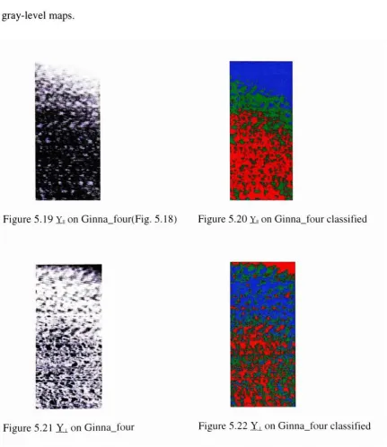
5.19

Y||OnGinna_Four

87

5.20

Y||

on

GinnaFour Classified

87

5.21

Y_l

on

GinnaFour

87

5.22

Yi

on

GinnaFour Classified

87

5.23

Image Band 48

from

a

400

by

400 Portion

of

C9

88

5.24

GinnaFour Image Band 45

88

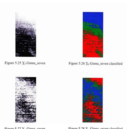
5.25 Y||Ginna_Seven

89

5.26

Yy

GinnaSeven Classified

89

5.27

Yi

Ginna_Seven

89

5.28

Yi

Ginna_Seven Classified

89

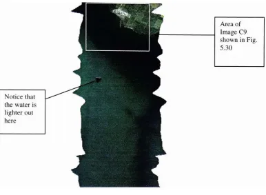
5.29

C9-R,G,B Image

of

Ginna

91

5.30 Smaller Portion

of

Image C9

Showing

Coastal Bottom Type

Variation

92

5.31

C2

-Along

Ontario Beach

and a

Spatially

Resized Portion

of

C2,

Ont_One

94

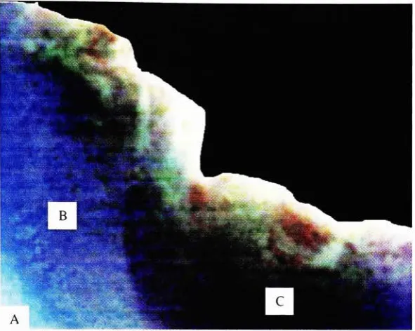
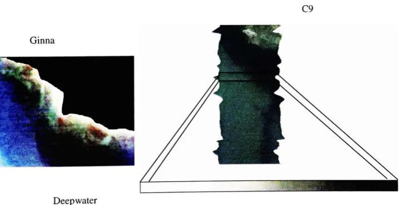
5.32 Image

Ginna

and

the

Deepwater Taken Over

the

Entire

Width

of

the

Image

95

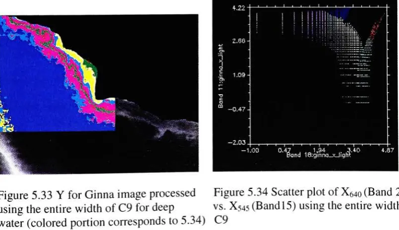
5.33 Y

for

Ginna Image Processed using

the

Entire Width

of

C9 for

Deep

Water

96

5.34

Scatter Plot

of

X640

vs.

X545 Using

the

Entire Width

of

C9

96

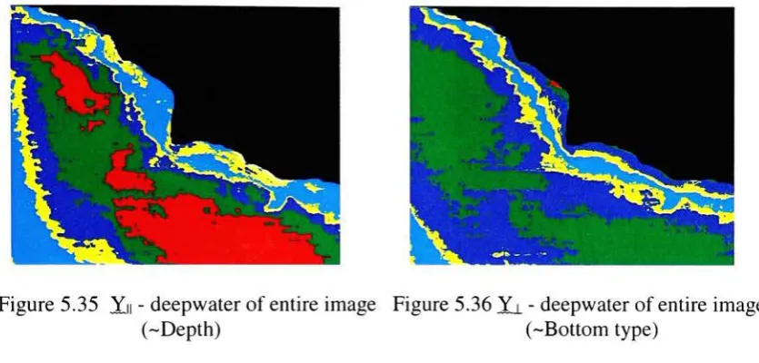
5.35

Yr

Deep

Water

of

Entire Image

(-Depth)

98

5.36

Yi-Deep

Water

of

Entire Image (-Bottom

Type)

98

5.37 Ginna Image

and

Deep

Water from

the

Right

Side

of

C9

99

5.38

Yy

for Ginna Processed With

Deep

Water

From Right

of

C9

100

5.39 Scatter Plot

of

X640

vs.

X545

Using

the

Right

Side

of

C9

for

Deep

Water

100

5.40 Eigenvalues from PCA

on

Ginna Image Processed

Using Deep

Water

from

the

Right Side

of

C9

101

5.41

Y|,

Using

Deep

Water from Right

(-Depth)

102

5.42

Y

Using Deep

Water from Right (-Bottom

Type)

1

02

5.43

Yi

(-Bottom

Type)

is

Picking

Up

on

Variations in Ginna Image

1 03

5.44 Image

and

Deep

Water from

the

Right

Side

of

Ginna

104

5.45 GinnaRight With Colors

Corresponding

to

5.46

104

5.46 Scatter Plot

of

X640

vs.

X545

for Ginna_Right

104

5.47

Y||

(-depth)

-

AT-means Classification

of

GinnaRight

Using

3

Classes

and

4

Classes,

Respectively

1 05

5.49

GinnaLeft

With

its

Corresponding

Depth

and

Bottom

Type

Maps

107

5.50 GinnaMiddle With

its

Corresponding

Depth

and

Bottom

Type Maps

1 07

5.51 Image Near

Ontario

Beach, C2,

and

the

Image

jArea

Selected

for

Processing,

OntOne

109

5.52

Yy

for

Ont_One

110

5.53

Yn

Classified

for OntOne

110

5.54

Yi

forOnt_One

110

5.55Yi

Classified for Ont_One

110

5.56

Ground Truth Results for OntOne

Ill

5.57 Transmission

and

Upwelled Radiance

for September

3,

1999

1 12

5.58 Plot

of

Sensor-Reaching

Radiance for

a

Zero-Reflectance

Bottom

113

5.59

Sensor-Reaching

Radiances

at

Depth

of

0.5

m

114

5.60

Sensor-Reaching

Radiances

at

Depth

of

1

m

114

5.61

Sensor-Reaching

Radiances

at

Depth

of

30

m

115

5.62 Eigenvalues

from

the

PCA

on

Model Data

116

5.63 Quantitative Depth Results for GinnaLeft

117

5.64

Quantitative Depth Results for GinnaRight

118

5.65 Quantitative

Depth Results for GinnaMiddle

118

6.1

C9 Image Near Ginna Power Plant

122

6.2

Y||-Deep

Water

of

Entire Image

(-Depth)

122

6.3

Yi-Deep

Water

of

Entire Image (-Bottom

Type)

122

6.4

Y||

Using Deep

Water From Right

(-Depth)

123

6.5

Yx

Using Deep

Water

From Right (-Bottom

Type)

123

6.6

Y||

(-Depth)

for Ginna_Right

124

6.7

Yx

(-Bottom

Type)

for

Ginna_Right

124

6.8

Smaller Portion

of

Image C9

(Ginna)

126

List

of

Tables

4.1

MISI Bandcenters for Visible

and

NIR

Bands

65

4.2

Inputs

to

HydroMod

72

5.1

Water

Sampling

Dates

and

Locations

-1999

and

2000

78

5.2

Sampling

Results for

Ginna,

September

3,

1

999

78

5.3

Ginna

(C9)

MISI Bands Retained

for

Algorithm

90

D.l

September

3,

1999

Chlorophyll-a

concentrations

-determined

Spectrophotometrically

1

67

D.2

September

3,

1999

Chlorophyll-a

values

-determined

Fluorimetrically

1

68

D.3

September

3,

1999 TSS Values

168

D.4

September

3,

1999 CDOM Values

169

Chapter 1

introduction

An

advantage

of

remote

sensing

is

that

it

provides a synoptic

view

and can

help

reduce

the

amount of

time

and

money

spent

on

sampling.

A

drawback

is

that

the

mtervening

atmosphere presents a challenge

to the

interpretation

of

remotely

sensed

images.

Remote sensing

over

water

is

a

particularly

difficult

task

because

the

water

is

an

additional

attenuation source.

Various

components

in

the

water act

as

absorbing

and

scattering

centers

for

the

radiation

that

penetrates

into

the

water

column.

Much

of

the

research

that

has

been

conducted on

remote

sensing

over

water

has

been

concerned

with

the

oceans.

Remote sensing

over

shallow water

adds one more

complexity

to

the

problem: reflection

from

the

bottom. The

radiance

reaching

the

sensor

over

optically

shallow water

includes

not

only

radiation

reflected

from

the atmosphere,

but

also

radiation reflected

from

the

surface of

the

water,

from

the

water column

itself,

and

from

the

bottom.

Understanding

the

properties of shallow water

is important

because many

recreational and economic activities

take

place near

shore.

Remote sensing is

a

tool that

can

be

used

to

understand

these

shallow

water

properties,

such as

bottom

type

variation

and

depth.

For

example,

Monroe

County

is interested in

the

location

and

distribution

of

Rochester,

NY. The Monroe

County

Environmental Health

Laboratory's

"1998 Ontario

Beach

Monitoring

Report"

states

that

decaying

algal plant

matter,

specifically

cladophora

and

spyrogyra,

was responsible

for

13%

of

the

beach

closures.

These

algae wash

up

on

shore where

they

act as a substrate

for bacterial

growth and provide

to the

bacteria

a

shield

from

the

harmful

effects

of

ultraviolet

light. In

coastal waters

there

is

a

relationship

between

high

levels

of

bacteria

known

as

indicator

bacteria,

which are

typically

found

in

the

presence

of

harmful

bacteria,

and

the

occurrences of

swimming-related

illnesses. The Health Lab is

interested

in

knowing

where

the

algae are

growing in

the

water

as part of

their

effort

to

manage

the

problem.

A

bottom

type

map,

produced

from remotely

sensed

data,

would

be

useful

in addressing

such

ongoing

environmental

problems.

The

algae

grow on

hard

surfaces,

such as

the

rock

comprising

parts

of

the

lake

floor

near

the

Ontario Beach

area.

The

rock and

algae

reflect

light reaching

the

bottom

of

the

lake

differently

than

the

surrounding sand,

which

is

the

reason

bottom

type

mapping

is

capable

of

distinguishing

between

a

rock

bottom

and a sand

bottom.

In

addition

to

providing bottom

type

information for

applications such as

the

one

discussed

above,

remote

sensing

of shallow

waters

can

also provide

depth information.

Photogrammetric

analysis of

the

bottom

of

Tampa

Bay

provided

information

about

circulation

patterns

in

the

bay

whichwas

extremely beneficial in

the

evaluation of

plans

for

dredging

the

bay

(Rosenshein

et

al.

1977).

However,

interpretation

of aerial

photographs

using

photogrammetry

is

limited

because

water

depth

variations are not

calls

for

a

technique

which will

distinguish

the

variation

in

bottom

type

reflectance

from

the

variation

in

the

reflectance spectra

due

to

absorption and

scattering

within

the

water

column.

This

is

the

problem addressed

in

the

current research.

This

research contributes

in

three

ways

to the

study

of

using remotely

sensed

imagery

to

gain

information

about

depth

and

bottom

type

in

shallow,

coastal

water.

First,

the

algorithm

used

here

was

implemented

on

a

hyperspectral image

taken

by

the

Modular

Imaging

Spectrometer Instrument

(MISI),

rather

than

a synthetic

data

set.

This involved

identifying

the

challenges of

using

real

data,

working

around

them,

and

analyzing

the

algorithm's

limitations

The

algorithm was

implemented

to

determine

qualitative

depth

and

bottom

type

information

from

images

taken

at

the

Ginna

power plant and near

Ontario Beach.

Second,

the

research shows

the

usefulness

of

the

bottom

classification

map

to the

County

Health Lab in

their

management

efforts

to

prevent

beach

closures

due

to

algae

washing

up

on

the

shore.

The

third

contribution

is

taking

Philpot's

algorithm

in

a

new

direction

by

using

principalcomponents regression

(PCR)

to

quantitatively

determine

the

unknowns

(depth,

bottom

type,

water

type)

that

combine

to

form

an

image

over

shallowwater.

This study illustrates how

the

radiative

transfer

model

HydroMod

can

be

used

as

a model

to

simulate

the

conditions under which

the

Lake Ontario

MISI

images

were

taken,

calculating sensor-reaching radiances,

which

were

then

used

to

Chapter

2

Background-Literature Review

2.1

Radiance

Reaching

the

Sensor

Remote

sensing

over

shallow

water

is difficult because

of

the

various components

that

contribute

to the

radiance

that

reaches

the

sensor.

There

are

essentially

two

components

that

make

up

the

sensor

reaching

radiance.

The

first is

the

upwelled radiance

scattered

from

the

atmosphere

(blue

arrow

in Fig. 2.1). The

second

is

the

radiance

reflected

from

the

scene,

composed

of

three

different

parts:

(1)

The

radiance reflected

from

the

surface of

the

water

(green

arrow

in

Fig

2.1),

(2)

water

column reflected

radiance

(violet line in

Fig

2.1),

and

(3)

bottom-reflected (orange

arrow

in

Fig

2.1).

The

radiative

transfer

model,

HydroMod,

can

be

used

to

understand

the

components

shown

in

Fig. 2.1. HydroMod

is

a

tool

for

calculating

radiance

distributions using

realistic environmental

conditions.

It

uses

the

Air

Force Laboratory's MODTRAN (Berk

1989),

one

of

the

most accurate radiative

transfer

computer

models

available, to

calculate

the

atmospheric conditions

through

which

photons

travel

on

their

path

toward

the

water

surface and

again

on

their

return

to the

sensor

(Fairbanks 1999).

The HydroMod

program

consists

of

four

modules

(Fairbanks 1999). The first

module

calculates

the

input

radiance

distribution using MODTRAN

to

calculate

atmospheric conditions.

The

second

module

involves

the

transition through the

water

surface

both

into

and

out of

the

water.

The

third

module

handles

the

propagationand

reflection underwater.

This

is

accomplished

using

Dr. Mobley's Hydro light

code

(Mobley 1995,1996)

to

solve

the

radiative

transfer

under

the

water.

Finally,

the

light is

propagated

back

through the

atmosphere

to

the

sensor

using

MODTRAN.

2.1.1

Atmospheric Attenuation

The

radiance

reaching

the

sensorover water

first

passes

through the

atmosphere

where some of

it

is

scattered and some of

it is

absorbed.

Direct

solar radiation

is

scattered

and

absorbed,

but

stillproceeds

from

the

general

direction

of

the

sun,

as

opposed

to

diffuse sky

radiation,

which results

from scattering

by

aerosols and air

molecules.

Bukata,

et

al.

(1995)

define

the

atmospheric attenuation

coefficient,

cs(A),

as

the

fraction

of radiant

energy

removedper unit

distance

due

to

absorptionand

scattering

summationof

the

attenuation

coefficients

due

to the

various

components

that

comprise

the

atmosphere.

Attenuation

by

the

atmosphere

is

a result of

molecular

(Rayleigh)

scattering,

aerosol

scattering,

and absorption

by

gases.

The

atmosphere

interferes

with

the

signal

from

the

water, requiring that

its

effect

be

removed

in

order

to

analyze

the

scene.

The

algorithm

implemented

here

on

MISI

images

subtracts

off

the

effect of

the atmosphere,

based

on

the

assumption

that the

atmosphere

is

invariant

over

the

scene,

in

a procedure

termed the

"deep-water

correction".

The

radiative

transfer

model,

HydroMod,

was

used

to

model

the

conditions under which

the

MISI

images

were

taken, resulting in sensor-reaching

radiance values.

2.1

.2

The

Air-Water Interface

Photons

not scattered

by

the

atmosphere

interact

with

the

watersurface.

At

the

surface,

they

are

either

reflected, refracted,

or

transmitted.

Refraction

of

the

light

is

governed

by

Snell's

Law,

na

sin

9a

=

nv

sin

Gv

(2.1)

in

which a and w refer

to

air and

water, respectively,

and n

is

the

index

of refraction.

The

angle,

6,

is

the

angle

between

the

direction

of

the

photon

flux

and

the

in-water

normal.

The

reflected photon

flux

is

given

by

Fresnel's

reflectance

formula. For

_tan2(fl,-flr)

11

tan2(0,+0f)

For

parallel polarized

light,

the

reflectance

is

(2.2)

_sin2(,-flr)

sin2(0,+0r)

P

=

-.2

(2.3)

And

for randomly

polarized

light,

5sin2(fl,-flr) |Q5tan2ffl-^)

sin2(#, +0,)

'

tan2(#,

+8r)

(2.4)

Further

information

on

the

air-_water

interface,

including

the

impact

of

waves,

is

given

in

Bukata

(1995)

and

Mobley

(1994).

2.1.3

In The Water

As

discussed,

the

atmospheric

and

water

surface

interactions

are accounted

for in

HydroMod (Fairbanks 1999). HydroMod

also accounts

for

the

in-

water

interactions,

but

the

water properties

are

required.

The

ground

truth

gathered

for

this

project allows

the

optical

properties

ofthe

water

to

be determined

and used as

inputs

to

HydroMod. The

Case 1

waters are

those

waters

that

have

a

high

concentration

of phytoplankton

compared

to

colored

dissolved

organic matter and nonbiogenic particles

or

where

the

phytoplankton

covary

with

the

other components.

Most

coastal

water

is

considered

Case

2

water

because inorganic

or colored

dissolved

organic matter

from

land drainage

are

important

and

may

not

covary

with

absorption

by

pigments,

such

as

chlorophyll

(Mobley

1994).

This

research

is

concerned

with

these

coastal waters.

The

concentrations

of

these

components

determine

the

optical properties ofthe

water.

There

are

two

different

categories of optical properties

-apparent and

inherent.

According

to

Mobley

(1994),

apparent

optical

properties are

those

properties of

the

water

that

depend

on

both

the

medium

and

the

structure of

the

light

field,

and

that

are regular

enough

to

provide

a

good

description

of

the

water.

Inherent

optical

properties are

those

properties

that

depend solely

on

the

medium.

2.1.3.1

Inherent Optical

Properties

The inherent

optical properties of water

include

the

absorption

coefficient

a(A),

the

total

attenuation coefficient

c(A), the

scattering

coefficient

b(X),

the

forwardscattering

probability

F(X),

the

backscattering

probability

B(X),

the

scattering

albedo

<o0(A),

and

the

volume

scattering function

(5(9)

(Bukata 1995). Definitions

of

these

properties are

taken

from

Mobley

(1994). Figure 2.2

shows

the

geometry

which will

be important in

defining

Od.)

<I)i/.i

>,</.!

Figure 2.2

Geometry

used

to

define

Inherent Optical Properties

(Mobley'

s

Fig

3.1)

Mobley

defines

a small volume

AV

of

water,

of

thickness

Ar,

which

is illuminated

by

a

narrow

collimated

beam

of

monochromatic

light

Oj(A.),

W

nm"1.

Part

of

this

incident

power

is

absorbed

by

the

water

volume and

is designated &a(A).

Also,

some part of

this

power

is

scattered

out of

the

incident beam

at angle

y/,

and

is

termed

0s(y/;A).

The

power

in

the

beam

that

has

not

been

either

scattered

or

absorbed

is

transmitted

0(A)

through the

volume

of water.

Assuming

that

no

inelastic scattering

occurs

and

the

photons

retain

their

original

wavelengths,

under

the

conservation of

energy,

<DJU)

=

Oa(A)

+

<DJ(A)

+

<D,(A)

(2.5)

The

spectral

absorbance,

A

(A),

is

that

fraction

of

incident

power

that

is

absorbed within

the

volume

defined

above.

Likewise,

the

spectral

scatterance,

B(A),

is

that

fraction

which

power,

which

is

transmitted through the

volume.

These

three

quantities are

mathematically

defined below:

<D,(A)

0,(A)

K

}

0,(A)

(2.6) (2.7)

(2.8)

The

inherent

optical properties are

the

spectral absorption coefficient

and

the

spectral

scattering

coefficient,

which

are

the

absorptance and scatterance

per unit

distance.

The

spectral absorption coefficient

is

a{A)=Yxm^-{m'x)

Ar->0

fij-The

spectral

scattering

coefficient

is defined

as

(2.9)

b{X)

=

lim

^

(")

a/-->o

Ar

(2.10)

The

total

beam

attenuation coefficient

is

the

summation

of

the

absorption

and

scattering

coefficients,

c(A)

=

a(A)

+

b(A)

(m~])

(2.11)

The

above

terms

describe

the

attenuationof

light propagating

through

water.

The

remaining inherent

optical properties

describe

the

directionality

of

the

scattering

the

angular

distribution

of

this

scatter:

the

angular scatterance per unit

distance

and

unit

solid

angle,

known

as

the

spectral volume

scattering

function is

given

by

i3{;A)

=

lim lim

^^

=

lim

lim

^'A)

(m^sr^)

Ar^om->o

ArAQ

Ar->oAn-o

0,(/l)ArAQ

(2.12)

where

AQ

is

a

given solid angle.

The

spectral

power

scattered

into

this

given

solid

angle

is

equal

to the

spectral radiant

intensity

scattered

into

the

direction indicated

by

\\>

times

the

given solid angle.

Therefore,

^;A)Slim

IAy/U)

^^E,(A)AV

(2.13)

which

gives

rise

to the

definition

that

the

spectral volume

scattering function

is

the

scattered

intensity

per unit

incident irradiance

per unit volume of water.

Irradiance

(")

is

defined

as

the

rate at which

the

radiant

flux,

or

power,

is delivered

to

a surface.

The

radiant

intensity (

/

)

describes

the

directional

information

about

the

flux (Schott 1997).

The relationship between

the

spectral volume

scattering function

and

the

scattering

coefficient

is defined in

the

following

formula

where

E

represents

the

unit

sphere.

K

b(A)

=

j/3(y/;

A)dQ.

=

In

\/3(y/;

A)

sin y/dy/

The

integration defined

above

is

typically

divided into forward

scattering,

over

the

angles

0

<

< 7i/2 and

backward scattering

over

the

angles rc/2 <

vj/<_n.

The

forwardscattering

coefficient,

bF,

and

the

backscattering

coefficient,

bB,

are

defined

as

follows

bF

=

2k

\/3(y/)

sin y/dy/ 0

,7

6fl

=

2;r

J

P(y/)

sin

^<i^

*d

(2.15)

(2.16)

Bukata

(1995)

explains

that

the

photons scattered

into

either

the

forward

or

backward

direction

are spoken of

in

terms

of

probabilities,

or

the

fractions

of

the total

scattered

flux

directed

into

each

hemisphere. The

forwardscattering

probability,

F,

is

the

ratio

of

flux

scattered

into

the

hemisphere

ahead of

the

incident

flux

to the

total

scattered

flux.

Similarly,

the

backscattering

probability,

B,

is

the

ratio of

the

flux

scattered

into

the

hemisphere behind

the

incident flux

to the total

scattered

flux

and

these

probabilities are

defined

in

the

following

equations.

F

=

^

B

=

^

b

b

(2.17) (2.18)

The last IOP introduced here

is

the

spectral

single-scattering albedo,

&>o,which

is

c(A)

(2.19)

2.1.3.2

Bulk

vs

Specific Inherent

Optical

Properties

Bulk

inherent

optical

properties

(IOPs)

are

those

that

are

described in

the

previous

section

and are

based

on

considering

the

water

column as

a

whole

rather

than

as

various

components

that

absorb and scatter.

Specific

inherent

optical properties

are

those that

are

attributed

to the

individual

components

in

the

water

that

act

as

absorbing

and

scattering

centers.

These

specific

IOPs

are

the

ones

that

must

be determined

when

trying

to

use

remote

sensing

to

determine

concentrations

of

the

various components

in

the

water.

The

bulk

IOPs,

previously

defined,

are

simply

summations of

the

individual

specific

IOPs.

From Bukataetal.

(1995),

a(A)

=

f^x,a,U)

1=1

bW^xMU

B(A)b(A)

=

fjx,B,WbM)

(2.20) (2.21) (2.22)

where

B(A)b(A)

=

backscattering

coefficient

at

wavelength

A (product

of

backscattering

probability

and

the

scattering

coefficient)

Xj=

concentration of

the

z'thcomponent

of

the

water column

at(A)

=absorption coefficient

at

wavelength

A for

a

unit

concentration of

bi(A)

-scattering

coefficient at wavelength

A for

a unit concentration

of

aquatic component

i

The

specific absorption coefficient and

the

specific

scattering

coefficient are

frequently

referred

to

as

the

absorption cross-section and

scattering

cross-section,

respectively.

Bukata

et al.

(1995)

states

that the

governing

principle

behind

the

remote

sensing

of

the

organic and

inorganic

components of

water

is

that

the

optical

cross

sections provide

the

link

between

the

concentrations of

the

individual

components

in

the

water and

the

bulk inherent

optical properties.

If

the

concentrations

of

the

individual

components

in

the

water

can

be

determined,

and

the

optical cross sections

of

the

water

are

known,

the

total

attenuation of

the

light

due

to

absorption

and

scattering in

the

water

column

can

be determined.

Bukata

et al.

(1995)

limit

their

optical

model

to

four

components,

which

are

followed

in

this

research.

A

comprehensive

model,

which

considers

the

optical

cross

sections of

every

aquatic

component

in

natural

waters,

is

unattainable.

Their

rationale

is

that

for

the

Great Lakes

waters,

only

a

small

loss in generality

occurs

due

to

using

this

four-component

model,

as opposed

to

a model which

includes

a

fifth

component,

non

living

organics, to

account

for detrital

matter.

These non-living

suspended organics

rarely

dominate

the

color

of

inland

and coastal waters.

The four-component

model

includes

pure water

(W),

chlorophyll

(Chi),

dissolved

organic carbon

(DOC),

and

a(A)

=

aw

(A)

+

xxaCM

(A)

+

x2aSM

(A)

+

x^^

(A)

b(A)

=

bw

(A)

+

xxbCM(A)

+

x2bSM

(A)

B(A)b(A)

=

Biy(A)bw(A)

+

xi

BCh, (A)bch, (A)

+

x2BSM

(A)bSM (A)

(2.23)

(2.24)

(2.25)

The

coefficients

x/, X2,

and

X3

are

the

concentrations

of

chlorophyll,

suspended

minerals and

DOC,

respectively.

The

absorption

cross-section and

scattering

cross

section

for

Lake

Ontario (Bukata

1995)

are shown

in Figures 2.3

and

2.4. Bukata

(1995)

makes reference

to

suspended

minerals,

but

this

component

will

be

referred

to

here

as

suspended matter

because

this

research

does

not

distinguish

the

mineral

from

the

organic

particles.

D 4-B SOD C

I-0S9OLVED DRGA^C O-JWO"

Cr*jO*0**m.

.j_

a-jC vn S5Q 0O 650 TOO

Figure

2.3 Pure

water absorption coefficient

and

absorptioncross-section

spectra

for

chlorophyll, total

suspended

mineral,

and

dissolved

organic carbon

indigenous

to

Lake

op o aoo mo oo 630 too

s

i

S

-00 ₅

-002

O*L0flQPLL 1

00 450 500 530 SOO Sao rao

Figure 2.4 Pure

water

scattering

coefficient and

scattering

cross-section spectra

for

chlorophyll and

total

suspended

minerals

indigenous

to

Lake

Ontario

(Fig

5.6

of

Bukata

1995)

In

order

to

generate

the

sensor-reaching

radiances,

HydroMod

requires

the

component

concentrations

for

chlorophyll,

suspended

solids,

and

DOC. These

component

concentrations

are

multiplied

by

the

optical cross-sections oftheaquatic components

included in

the

model.

Updated

opticalcross-sections

for

these

components

in Lake

Ontario,

determined from processing

and

analysis

of water

samples,

are

included in

the

HydroMod

model

to

generate radiance

data,

with

the

exception

of pure water and

chlorophyll.

These

updated cross-sections

are

presented

in Section 2.2.

2.1.3.3

Apparent Optical Properties

As

stated

earlier, the

apparent optical properties

(AOP)

depend

not

only

on

the

radiometric

quantity

other

than

radiance

is

used.

The

first

AOP

that

will

be discussed

here

is

the

irradiance

attenuation

coefficient,

K(Az). Bukata

et al.

(1995)

define

the

irradiance

attenuation

coefficient as

the

logarithmic depth

derivative

of

the

spectral

irradiance

at a

depth

of

z.

The

actual

definition

of

K(X

z)

results

from Beer's Law

(Bukata

1995)

and

is

derived below. A beam

of

light passing

through

a medium

loses

some

of

its initial

radiance

flux

value,

0mc,

due

to

absorption

loss

by

an

attenuating

medium of

thickness

Ar,

and

only

0trans

remains of

the

original

beam

of

light,

according

to the

following

form

of

Beer's

law.

O

-O

=-oO

Ar

trans mc mc

(2.26)

or

AO

=_-amcAr

(2.27)

The

constant of

proportionality,

a,

is defined

as

the

absorption coefficient.

Then,

in

the

limit

as

both

AcPand Ar

approach

zero, the

equation

becomes

d

=_-adr

O

which

is

Beer's Law.

Integrating

equation

2.28

from

r=

₀

to

a

distance

r

in

the

absorbing

medium,

and

knowing

that

the

beam

coefficient

is

a

function

of wavelength

yields

the

following

equation:

<S>(r,A)=(0,A)e-aU)r

(2.29)

and

consequently for

a

beam

propagating vertically in

water,

E(A,

z)

=

E(A,0

~)exp[-K{A,

z)z]

(2.30)

where

E(Az)

=

the

value of

irradiance

at

depth

zand

E(AO-)

=

the

irradiance just below

the

air-_water

interface.

Finally,

Equation 2.31 defines

the

irradiance

attenuation

coefficient,

resulting from Beer's Law

being

used

to

describe

the

attenuation of spectral

irradiance

with

depth

z

(Eq.

2.30).

K(A,z)=

'

E(A,z)

6E(A,z)

dz

(m'1)

(2.31)

This AOP

shows

how

the

irradiance decreases

exponentially

with

depth

due

to

downwelling

irradiance

attenuation coefficient

Kd(Xz)

and

the

upwelling

irradiance

attenuation coefficient

Ku(Xz)

is

40U)

(2.32)

(2.33)

where

Ed

and

Eu

refer

to

the

downwelled

and upwelled

irradiances,

respectively.

For

a

review

of

these

radiometric

terms,

refer

to

Schott (1997).

2.2 Composition

of

Natural Water

Natural

waters

are composed

of a

myriad of

living,

non-living,

and

once-living

material.

These

components

determine

the

optical properties

of

the

water

that

were

discussed in

the

previous section

2.2.1 Pure Water

Pure

water

implies

that the

water

is free from

the

scattering

and absorption effects

of organic

and

inorganic

matter.

The

attenuation

due

to

pure

water

is due only

to

water

molecules.

Pure

water

typically

absorbs

weakly in

the

blue

and green

regions of

the

electromagnetic

spectrum.

As Kirk

(1983)

states,

the

absorption

of pure water

increases

above

550

nm

and

is

quite significant

in

the

red.

Figure

2.5

shows

the

absorption and

scattering

spectra of pure

water

as

measured

by

Smith

and

Baker

(1981),

which are

the

Water

290 340 390 440 490 540 590 640 690 740 790 840 890 940 990

Wavelength

(nm)

-_Absorption

Scattering

Fig. 2.5 Optical Properties

of

Pure Water (Smith

and

Baker

1981)

Above

550

nm,

the

attenuation of

light

by

pure water

is dominated

by

absorption and

the

total

attenuation

coefficient

due

to

pure water can

be

approximated as

the

absorption

coefficient

due

to

pure

water.

However,

in

the

blue

region,

A

=

400-520

nm,

scattering

by

pure

water

plays a

greater

role

in

total

attenuation

(Bukata 1995). The strong

absorption

in

the

red and weak

absorption,

but strong

scattering,

in

the

blue-green

region

of

the

spectrum causes

the

blue

appearance

of

water.

2.2.2 Dissolved

Salts

and

Gases

Dissolved

salts and gases are not

included

in

the

four-component

model

discussed

earlier.

Dissolved

salts

do

affect absorption within

the

water

column,

with

the

most

significant effect at

ultraviolet

wavelengths,

A

<

300

nm.

Molecular

scattering

in

compared

to the total

attenuation.

The

specific

directional

scattering due

to

pure

water/dissolved salts plays a more significant role

in

molecular scattering.

However,

for

inland

waters,

the

ability

of

dissolved

salts

to

create a

directional

nature

to

/3(y/)

is

significantly

reduced compared

to

mid-oceanic waters

due

to their

much

lower

concentrations

in

fresh

water

(Bukata 1995).

Dissolved

gases,

of

which

dissolved

oxygen

is

the

most

significant,

also

do

not produce significant changes

to

the

bulk

optical

properties

of

the

water,

and

therefore,

are

not

included

in

the

model.

2.2.3

Dissolved Organic Matter

Dissolved

organic matter

(DOM)

does

not

have

a

significant

impact

on

scattering

as evidenced

by

the

fact

that

it is

not

included

in Eq. 2.24. DOM

does, however,

impact

the

absorption

in

natural waters and

is

often

the

dominant

component

in

the

optical

absorption

of coastal water

(Vodacek

et al.

1997). The optically

active

component

of

DOM

is

referred

to

as

Colored Dissolved Organic Matter (CDOM). DOM is

a result of

excretion, secretion,

or

decomposition

of

plants and animals

in

the

water,

or of

direct

input

of

terrestrial

material.

Plant

or animal

materials are

transformed

into DOM

through

hydrolysis,

photolysis,

and

bacterial

decomposition

of

their

cellular

structure.

The

decomposition

of

plants and

animals results

in

water

soluble

humic

substances

which are

responsible

for

the

yellow color observable

in

some

inland

and coastal

waters.

Although

these

pigments comprise

only

about

40%

of

the

DOM,

the

yellow

hue has

given rise

to

the

various

terms

given

to

DOM,

such

as

colored

dissolved

organic matter

(CDOM),

Lake

Ontario displays DOM

concentrations

on

the

order of

2 g

C/m3,

which

is

fairly

low

compared

to

average

lake

water

concentrations

reported

in

the

literature

of

9

or

10 g C/m

.

(Bukata

1995)

An

absorption curve can

be

represented

by

the

following

relationship,

which

is

valid over

the

wavelengths

A

=

350-700

nm,

ag(X)

=

ag(Ao)

exp[-S(X-Ao)]

(Bricaud,

et all

981) (2.34)

The

subscript, g,

stands

for

gelbstoff.

The

variable,

S,

is

a

slope

parameter

assumed

to

be

independent

of

wavelength.

The

values

for

the parameter,

S

(nm"1),

typically

range

between 0.010

to

0.020,

with

a

mean value of

0.014. The

reference

wavelength,

Xq,

is

typically

arbitrary,

but usually in

the

UV

or

blue.

Spectrophotometric

analysis

of

a

water

sample,

filtered

to

remove

scattering

particles,

with

the

absorption

of

pure

water, subtracted,

becomes

an

estimate

of

ag(A).

The study

examined

the

wavelengths

between

A

=

350-700

nm

because

that

was

the

range

of

the

spectrophotometer

used.

Below A

=

350-700

run, there

were a

few discontinuities in

some

of

the

samples

measured,

but

the

absorption

between A

=

350

nm

and

A

=

700

nm

reasonably

followed

the

law

shown

in Eq.2.34. The

normalized

CDOM

spectral

absorption coefficient

of

Lake Ontario

water

(Fig.

2.6)

used

for

this

study in

the

HydroMod

model

was

determined from

samples collected on

May

20,

1999. A

spectral

absorption coefficient normalized

to

one at

350

nm

is

used

in

the

work

instead

of

a

coefficient

is

multiplied

by

a scalar

to

arrive at an

appropriate

spectral absorption

coefficient.

The

scalar used

for

Lake

Ontario

waters was

0.2.

CDOM

3.5

2.5

T 2

E

1.5

250 450 650

Wavelength

(nm)

850

-Absorption

Coefficient

Figure 2.6 CDOM

normalized spectral absorption coefficient used

in HydroMod

2.2.4

Suspended Matter

The

term

"suspended

matter"

includes both

organic and

inorganic

matter.

Suspended

matter

is derived from

plankton,

detritus from

the

decomposition

of

phytoplankton,

zooplankton,

and macrophytic

plants,

as well as

terrigenous

suspended

particles

formed

by

erosion and

discharge. A large

portion of

this

suspended

matter

is

suspended

minerals,

which

according

to

Bukata

(1981)

have

concentrations

in Lake

Ontario

of

0.2-8.9

g/m3.

The HydroMod

absorption and

scattering

cross-sections

for

suspended matter are

shown

in Fig. 2.7. The

absorption cross-section

was generated

from

a curve

that

represents

the

average of a set of curves

measured

from

water

samples

cross-section curve measured and modified

by

Dr.

Vodacek

to

match

Bukata'

s

(1995)

curve.

Suspended Minerals

290 340 390 440 490 540 590 640 690 740 790 840 890 940 990

Wavelength

(nm)

-Absorption

Scattering

Figure 2.7 Suspended Matter Absorption

and

Scattering

Cross-Sections

in HydroMod

In

addition,

there

are

various

precipitates,

a result of chemical

activity, that

can

affect

the

absorption

and

scattering

within a

water

body. For

example,

Landsat

first

viewed chemical

precipitations

of

calcium

carbonate,

known

as

whitings,

in

the

Great

Lakes in 1973

(Strong,

1978).

As

surface waters

become

saturated with

Ca"""

ions in

the

summer

time,

a

biological

or

physical mechanism

initiates

the

whiting.

Zooplankton feed

on

the algae,

detritus,

and

bacteria,

and

therefore

help

to

determine

the

status of

the

water.

For

example,

a

highly

productive water

body

will

have

a

higher

concentration

of

zooplankton,

while

the

populations

of zooplankton

in

natural

the

availability

of

food,

and

other

factors.

The

effect of zooplankton

on color

is

largely

unknown,

but

assumed

to

be

minor

due

to their

small concentrations

in

comparison

to

phytoplanktonand

bacterioplankton.

There

are also

bacterioplankton

in

the

water,

which

do

not

contribute

to

the

overall water

color,

although

they

probably have

some

effect on scattering.

Planktonic

fungi

are

colorless,

chlorophyll-

free lower

plant

forms

consisting

of cellular

filaments

containing

spores.

These

planktonic

fungi

present

in

the

watercolumn are assumed

to

have

negligible optical

impact

on

the

optical properties of

the

water

due

to their

lack

of

color

in

addition

to their

low

concentrations

(Bukata

1995).

2.2.5

Algal

Pigments

Phytoplankton

cells contribute

to

water

color,

depending

on

their

pigments.

All

phytoplankton contain chlorophyll and

carotenoids,

whichare responsible

for

photosynthesis.

All

greenalgae containchlorophyll

a,

and

possibly

b

and/or c.

As

Bukata

states

(1995),

the

ratio

of chl a

to

chl

b is

approximately

3:1,

and

therefore,

as

Bukata does in his

model,

the

research

here focuses

on

the

presence of chl a.

Chlorophyll

absorption occurs

in

the

blue

and red regions of

the

spectrum

(Fig.

2.8),

and

is

more

Chlorophyll

290

340 390

440

490 540 590

640 690

740 790 840

890

940 990

Wavelength

(nm)

-Absorption

?Scattering

Figure 2.8 Chlorophyll

a

Absorption

and

Scattering

Cross-Sections in HydroMod

(Bukata

1995)

Decomposed

chlorophyll,

in

the

form

of

phaeophytin,

must

be

accounted

for

because

it

causes

a

peak

shift

toward

shorter

wavelengths

in

the

blue

region and a peak

shift

toward

longer

wavelengths

in

the

red region.

The

intensity

of

the

absorption

for

this

chlorophyll

derivative is

weak compared

to the

intensities

of

the

absorption

bands

of

chlorophyll,

but

an

estimate

of

phaeophytin

is

essential

to

determining

the

portion of non

living

phytoplankton

in

the

water.

Understanding

these

properties

helps

in derivation

of algorithms

for

determining

2.3

Shallow Water Reflectance

The

irradiance just below

the

surface

includes

the

flux

scattered

back

by

the

water

column

itself

(i.e.,

the

photons

that

never reach

the

bottom)

and

the

flux

scattered

back

from

the

bottom:

Eu(0)

=

[Eu(0)]c+[Eu(0)]B

(2.35)

where

Eu(0)

=

the

upwelling

irradiance just

below

the

surface

[Eu(0)]c

=

upwelling

irradiance just

below

the

surface

due

to the

water

column

[Eu(0)]b

=

upwelling

irradiance just

below

the

surface

due

to the

bottom

The derivation

of

the

following

expression

for

shallow

water

reflectance

is

included

in

Maritorena

et al.

(1994),

who use some

simplifying

assumptions

in

order

to

derive

analytical

formulas for

shallow water reflectance.

In

order

to

estimate

the

irradiance

due

to the

water

column,

they

model an

infinitely

thin

layer

of

thickness

dz

at

depth

z,

where

the

downwelling

irradiance

at

this

point

is

Ed(z)

.

The

backscattering

coefficient

for

this

downwelling

light

is

bbd-

Then,

the

upwelling

irradiance

created

by

this

infinitely

thin

layer

of

water

is

dEu(z)

=

bbdEd(z)dz

(2.36)

Ed(z)

=

Ed(0)exp(-Kdz)

(2.37)

where

Ed(0)

is

the

downwelling

irradiance

at zero

depth

and

Kd

is

the

downwelling

irradiance

attenuation coefficient.

The upwelling

irradiance is

also

attenuated;

this

attenuation

is

expressed

by

(-kz),

where

/cis

the

vertical attenuation