by
Alireza Adi, B.Sc. (Ag.)
A dissertation submitted in partial fulfilment of the requirements for the Degree of Master of
Agricultural Development Economics at the Australian National University
D E C L A R A T I O N
Except where otherwise indicated, this dissertation is my own work.
A. Adi
ACKNOWLEDGEMENTS
This study was carried out while I was a student at the
Australian National University, Canberra, on a Colombo Plan Scholarship offered by the Government of Australia and a scholarship offered by the Agricultural Development Bank of Iran. I am grateful to the Governments of Australia and Iran for their generosity.
I must acknowledge the large intellectual debt that I owe to my supervisor, Dr Peter J. Lloyd, of the Research School of Pacific Studies, Australian National University, who carefully read through all the drafts and made a great number of useful comments and suggestions. He placed his own knowledge in this field at my disposal. To him I owe a profound debt of gratitude.
I must acknowledge my sincere gratitude to Dr Dan Etherington, the Convenor of the Master's Degree Course in Agricultural Development Economics, Research School of Pacific Studies, Australian National University. His advice and guidance were a great encouragement for this study.
The suggestions and assistance of Dr Mark Saad, of the Development Studies Centre, Australian National University in this work are greatly appreciated.
I also would like to thank Miss Yvonne Pittelkow of the
Computer Centre, Australian National University and also Mr Julian Morris of the Industries Assistance Commission, Canberra, for their help in computing parts of this work.
My thanks also go to Mr Alan McDonald, Development Studies Centre, and the staff of the typing pool, Development Studies, Centre, Australian National University, who did the typing of the initial draft.
Canberra August 1977
This study attempts to review the basic principles of the consumer demand theory in order to estimate the demand for tea and coffee in Australia. Generally the study of consumer demand theory is
important because it can be used in development and production planning.
Some of the commonly used systems of demand equations for empirical studies are explained. The study also attempts to explain a habit formation hypothesis and incorporate the hypothesis in the systems of demand equations. On this basis, three models of demand equations with and without habit formation are used to estimate the demand for tea and coffee in Australia.
It is shown that none of the models satisfy all the general restrictions imposed on demand equations, since each one has some advantages and some disadvantages. However, through the comparison of these models it is shown that a habit formation model is justified. Tea in the Australian consumption pattern is an inferior good while
CONTENTS
Page
ACKNOWLEDGEMENTS (iii)
ABSTRACT (iv)
LIST OF TABLES (vi)
CHAPTER
1 INTRODUCTION 1
2 A BRIEF SURVEY OF DEMAND THEORY 10
2.1 Introduction
2.2 Consumer 10
2.3 The Nature of the Utility Function 11 2.4 Existence of the Utility Function 13 2.5 The Rate of Commodity Substitution 14
2.6 The Maximization of Utility 15
2.7 Ordinary Demand Functions 17
2.8 Compensated Demand Functions 19
2.9 Prices and Income Elasticities of Demand 21
2.10 Indirect Utility Functions 22
2.11 Additivity and Separability of Utility
Functions 24
2.12 Substitution, Complementarity and
Independence 26
2.13 Proposed System of Demand Functions 28 A - The System of Double Logarithmic
Functions 29
B - The Indirect Addilog System 29 C - The Linear Expenditure System 31 D - Transcedental Logarithmic Utility
Functions 34
CHAPTER Page
3 HABIT FORMATION MODELS 41
I - Stone-Geary Utility Functions 49
II - The System of Double Logarithmic Functions 52
III - Indirect Translog Functions 53
4 EMPIRICAL RESULTS 55
4.1 Introduction 55
4.2 Stochastic Specification and Empirical Results 57
The Data 57
I - Double Logarithmic System 59
II - Linear Expenditure System 69
III - Homogeneous Indirect Translog Functions 75
5 CONCLUSIONS 81
BIBLIOGRAPHY 84
TABLE
4 .1
4.2
4.3
4.4
4.5
4.6
LIST OF TABLES
TITLE Page
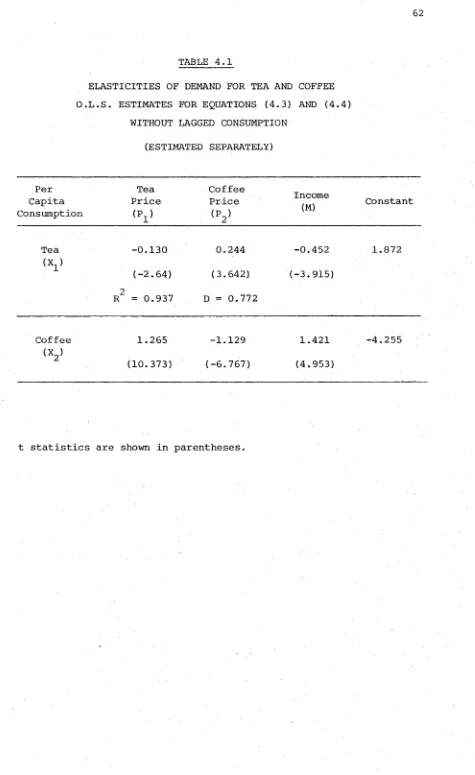
Elasticities of Demand for Tea and Coffee. O.L.S. Estimates for Equations (4.3) and (4.4)
Without Lagged Consumption. 62
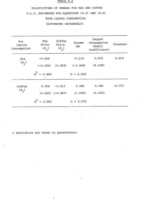
Elasticities of Demand for Tea and Coffee. O.L.S. Estimates'for Equations (4.5) and (4.6)
With Lagged Consumption. 63
Elasticities of Demand for Tea and Coffee. Maximum Likelihood Estimates for the Sub-System of Linear Expenditure System. Equations (4.7)
and (4.8) Without Lagged Consumption. 73
Elasticities of Demand for Tea and Coffee. Maximum Likelihood Estimates for the Sub-System of Linear Expenditure System. Equations (4.9)
and (4.10) With Lagged Consumption. 73
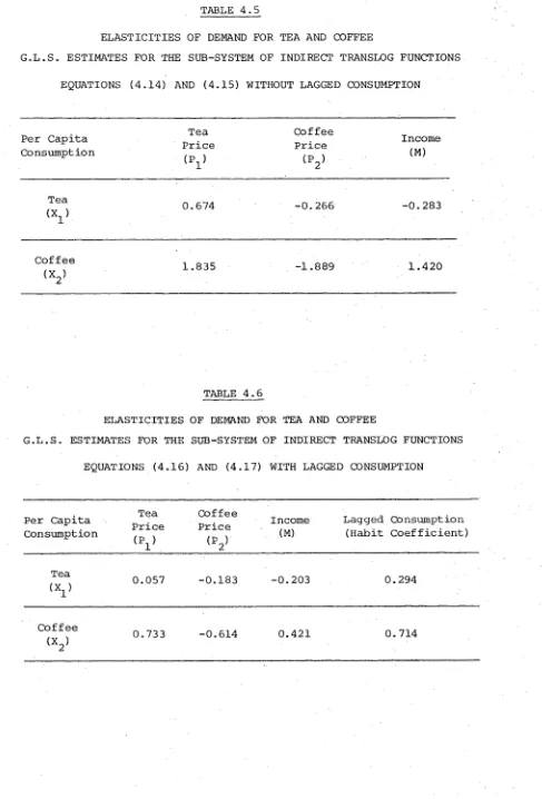
Elasticities of Demand for Tea and Coffee. G.L.S. Estimates for the Sub-System of Indirect Translog Functions. Equations (4.14) and (4.15)
Without Lagged Consumption. 79
Elasticities of Demand for Tea and Coffee. G.L.S. Estimates for the Sub-System of Indirect Translog Functions. Equations (4.16) and (4.17)
With Lagged Consumption. 79
CHAPTER 1 INTRODUCTION
The concern of this study is to investigate consumer demand theory and its application to commodities such as tea and coffee. There are two primary reasons for this investigation. The first point
is related to development planning and the second to production planning. Many countries are now engaged in construction of development programs and to do this adequately it is clearly necessary to have some idea about the changes in consumption that are likely to occur with rising income levels.
The structural transformation of the Japanese economy in the 1950's was reflected in the beginning of the absolute decline in the agricultural labour force and in the emergence of a highly sophisticated
industrial complex in Japan. This transformation coincides with the radical changes in food consumption patterns of Japanese people. As the real incomes grew rapidly, the institutional and technological
framework of Japanese life in general also changed rapidly. Under these circumstances, a drastic transformation took place in methods of food preparation and the patterns of food consumption.
To my mind the Iranian economy has been undergoing a similar path to the Japanese economy. The rapid rate of growth of the last decade following the land reform and transformation of the agricultural labour force to industry is bringing about a tremendous change in con sumption patterns of Iranian people. This has been especially true during the last few years as a general increase in the standard of
living was achieved by an increase in oil revenues.
I believe this study will enable me to learn the basic con cepts of consumer demand theory and its application to the Iranian economy at a proper time and with available data.
Secondly, from a production point of view, there is also a sound justification for this case study. In later chapters changes in consumption patterns due to changes in tastes and habit formation will be investigated. The theory will then be applied to the demand for tea and coffee in Australia. These two commodities, which are mostly produced in developing countries, are traditional commodities
used to drinking them. From the producers' point of view it is important to know the short and long run price and income elasticities of a commodity especially when a factor such as habit formation determines the consumption.
In the history of demand analysis two threads, related but separate, can be discussed. These are, first, the work of economists interested in the discovery of general laws governing the operation of individual commodity markets, particularly agricultural markets; and, second, the work of those interested in the laws or behavioural regular ities governing what has come to be called consumer preference.
Throughout the eighteenth and nineteenth centuries the empiri cal approach had made little or no progress in the measurement of demand curves despite its early and promising beginning. In a large part, this was due to the fact that the techniques of regression analysis were not developed by statisticians until late in the nineteenth century. Signi
ficant progress was, however, made in the investigation of the influence of income on consumption patterns. In particular, an outstanding con tribution was made by Engel who, in 1857, formulated what turned out to be enduring empirical laws governing the relation between income and particular categories of expenditure.
It was no accident that agricultural commodities were the first to be studied and indeed have provided econometricians with some of their most convincing successes. For partial equilibrium analysis based on fitting single equations requires, ideally, a homogeneous commodity with a simple quantity dimension, stable consumers' prefer ences, and relatively large fluctuations or trends in supply which are independent of the current market price; and these conditions are most nearly met by many agricultural staples.
By 1939 most of the strengths and weaknesses of what is called classical demand analysis had been probed and most of the techniques still in use had been discovered. It is possible to characterize this classical approach as consisting of the applica tion of variations in least squares single-equation fitting, to both time series and cross-section data, of market models based as far as possible on the theoretical results of Slutsky, Allen and Hicks. Much of this work, together with a great deal of empirical analysis, was drawn together by Shultz in 1938. However, because of the Second World War it was not until the 1950's that fully systematic treatments of this approach were published. The books by Wold and Stone can be regarded as a consolidation of the theoretical and empirical work on static demand models in the first half of this century.
Although there have been a number of important theoretical advances, on the empirical side, certain topics stand out clearly as
o f t h e m o r e s o p h i s t i c a t e d c o m p u t a t i o n a l a n d e c o n o m e t r i c t e c h n i q u e s w h i c h h a v e s i n c e b e c o m e a v a i l a b l e .
W h i l e t h e q u e s t i o n a s t o w h i c h t h e c l a s s i c a l a p p r o a c h
a d d r e s s e d i t s e l f w a s o f t h e t y p e " w h a t i s t h e i n c o m e o r p r i c e e l a s t i c i t y o f g o o d X ? ", m o re r e c e n t i n v e s t i g a t i o n s h a v e p o s e d a n d b e g u n t o a n s w e r
some m o r e f u n d a m e n t a l q u e s t i o n s ; f o r e x a m p l e , how s h o u l d dem and f u n c t i o n s b e s p e c i f i e d ? W hat i s t h e b e s t way o f a l l o w i n g f o r c h a n g e s i n p r i c e s ? W hat o t h e r i m p o r t a n t f a c t o r s s h o u l d b e c o n s i d e r e d i n a d d i t i o n t o i n c o m e a n d p r i c e ? I n p a r t i c u l a r , a t t e n t i o n h a s f o c u s s e d o n t h e t h e o r y o f dem an d a n d i t s r e l e v a n c e t o a p p l i e d dem and a n a l y s i s . I n t h i s c o n t e x t dem an d t h e o r y i s r e g a r d e d n o t a s p a r t o f g e n e r a l e q u i l i b r i u m a n a l y s i s o r o f w e l f a r e t h e o r y , b u t a s a t o o l o f e m p i r i c a l i n v e s t i g a t i o n .
considerable importance; the increase in the number of large econo metric models and the general increase in interest in models for planning and policy formulation offers a wide area for the positive application of any results which are achieved. Consumers' expenditure is the largest item in the gross domestic product of most economies and thus the usefulness of disaggregated planning or prediction is likely to depend on its correct allocation. The changing structure of industry over time depends crucially on the evolution of the elements of consumers' expenditure in response to increasing income while know ledge of price responses is an important element in the formulation of fiscal policy or any other type of economic control.
For some practical purposes it may be sufficient to estimate separately a set of single equation models, one for each category of consumers' expenditure. For example, each equation might express the
quantity purchased of each good per head of population as a function of average per capita income, the price of the good relative to some overall price index, time as a catch-all for changes in the distribu tion of income, the introduction of new products and steady changes
referred to as a "pragmatic" approach. It is pragmatic in the sense that it includes those variables in which one is directly interested, ignoring or summarising others.
However, there are a number of difficulties with such a treatment. For example, one assumption in the double logarithmic model is that the elasticities are the same at all values of the
exogenous variables. Although this is convenient, one should not expect it to be true over any but the shortest range, and when working with time series, for econometric purposes, one should like his time span to be as long as possible. Typically, nations become richer over time and one might expect goods which are usually luxuries when the inhabit ants of the country are poor to become more and more necessities as real incomes increase. But there is an even more basic problem: if all income elasticities were really constant, those goods with elastici ties greater than unity would, as real income increased, come to dominate the budget and eventually would lead to the sum of expenditures on each of the categories being greater than the total expenditure allocated, an obvious absurdity, i.e. it violates the budget restraint of consumer demand theory. Even if the model fits the data well when estimated, one knows that if it is used to project forward it will eventually lead to silly results. Obviously one needs a model with changing elasticities and one needs some theory of how one might expect them to change.
are unlikely to be reproduced in the aggregate. However, it could be argued that one "representative" consumer might represent the whole population. One might then write the demand function so that the aggregation difficulties are met and such that the elasticities for each good change in a sensible way. Even now, there are strong re strictions on the type of behaviour allowed. For example, if income and all prices were to change by the same proportion, real income and relative prices would not change and the quantities bought would remain the same. Although this absence of money illusion is an attractive property for demand functions to possess, it may not be true. Con
sumers may suffer from a money illusion and it could be argued that it is part of the task of demand analysis to discover whether or not it exists rather than to use a model which precludes it (as a starting point).
The choice of the demand model itself has important implica tions; strong a priori notions are built into the analysis by the choice of model and these will interact with the data to yield results which will be affected by the model chosen. At the same time such
strong preconceptions are inevitable; some functional form must serve as a basis for estimation, and even then when it has been chosen it will, in most circumstances, be possible to estimate only a few para meters for each commodity. This constraint, which is due to the lack of independent variations between prices and income in most time series, rules out the possibility of overcoming some of the specification
turned to the theory of demand as a tool for deriving the necessary constraints and for organising their a priori assumptions. A model based on preference theory usually offers a practicable alternative to the pragmatic approach and it is this alternative which has been most extensively explored in recent years.
CHAPTER 2
A BRIEF SURVEY OF DEMAND THEORY
2.1 Introduction
The theory of demand has been surveyed by many economists and there are several good references such as Brown and Deaton (1972), Green (1971) and Phlips (1974). However, in this chapter I will review the stochastic demand functions for a single commodity, say tea or coffee, which are my interest. To begin with, properties of utility functions are discussed.
Although the economists of the nineteenth century explained consumer behaviour on the assumption of cardinal utility functions, it was only a few decades ago that the consumer was assumed to be capable of only ranking commodity combinations consistently in order of
preference: Slutsky (1919); Hicks and Allen (1933). This means that the consumer's utility function is not unique. If a particular function describes (approximately) the consumer's preferences, so does any other function which is a monotonic transformation of the chosen function.
It is assumed that the utility function which represents these preferences is strictly quasi-concave, that is, sets such as {X; X R y} are strictly convex where X and Y are commodity bundles, and R is a weak preference relation. This ensures that the equilibrium
is a maximum and is unique.
he has a limited income. The necessary conditions for this maxi mization will be explained.
The consumer's ordinary demand functions for commodities will be derived from his first order conditions for utility maximi zation. In general, the quantities demanded of a commodity are a function of all consumer commodity prices and consumer's income. Ordinary demand functions are single valued and homogeneous of degree zero in prices and income. That is, we do initially assume that there is no money illusion. The consumer's compensated demand functions for commodities are constructed by changing his income following a price change in order to leave him at his initial utility level. The com pensated demand functions state quantities demanded as a function of all prices and the chosen level of utility. They are also single valued and homogeneous of degree zero in prices.
The consumer's reaction to price and income changes in terms of substitution and income effects will be analyzed. Substitutes and
complements will be defined in terms of the sign of the substitution effect for one commodity when the price of the other changes.
The chapter will finish by explaining other characteristics of utility functions such as additivity and separability and, finally,
some of the systems of demand equations which are frequently used in empirical studies will be mentioned.
2.2 Consumer
The postulate of rationality is the customary point of departure in the theory of the consumer's behaviour. The consumer is assumed to choose among the alternatives available to him that which is preferred to all others within the budget. This implies that he is aware of the alternatives facing him and is capable of evaluating them. All information pertaining to the satisfaction that the consumer derives from various quantities of commodities is contained in the utility function.
2.3 The Nature of the Utility Function
Consider the case that an individual consumer purchases a set of commodities. His ordinal utility function is
U = f(x , x , ..., x ) (2.1)
1 2 n
where (x,, x„, ..., x ) is the vector of quantities consumed of the
1 2 n
commodities 1, . .., n. It is assumed that (2.1) is a continuous
function and has continuous first and second order partial derivatives.
i.e. because it leads to the operational hypotheses which turn out to be valid. Its justification lies in the conclusions that can be derived from it".
The utility function is defined with reference to consumption during a specific period of time. The level of staisfaction that the consumer derives from a particular commodity bundle (or set) depends upon the length of the period during which he consumes it. There is no unique time period for which the utility function should be defined. However, there are restrictions upon the possible length of the periods. An intermediate period is most satisfactory for the static theory of consumer behaviour. This is because if the period is too short the con sumer cannot derive utility from variety in his consumption and diver sification among the commodities he consumes. On the other hand, tastes
(the shape of the function) may change if it is defined for too long a period. Hence, a period such as, say, from one quarter to a year is usually satisfactory.
2.4 Existence of the Utility Function
It is not obvious that real-valued functions that can serve as utility functions exist for all consumers. Consumer preferences must satisfy certain conditions in order to be represented by a utility
function. One set of conditions for the existence of a utility function is as follows:
Axiom 1 (completeness):
For all A^ and A^ in S (set of all commodity combinations), either A^ R A^ or A^ R A^ or both (R is regarded as "at least as good a s " ) .
Axiom 2 (transitivity):
For all A , A 2 , A 3 in S if A^ R A 2 and A 2 R A 3 (A1 R ^ R A ) , then A n R A .
1 3
Axiom 3 (rational choice):
If A^ is chosen from a set of alternatives S, then for all A2 in S, A x R A 2 .
2.5 The Rate of Commodity Substitution
Consider the simple case where
U = f (X) X = (x f x , . . . , x ) (2.2)
1 2 n
The total differential of the utility function is
dU = Zf.dx. (2.3)
l l
varying only quantities of two commodities i, j
d U = f . d x . + f . d x . (2.4)
i i 3 3
by variation in and x_. is approximately the change in x^ multiplied by the change in utility resulting from a unit change of x^ plus the change in x_^ multiplied by the change in utility resulting from a unit change in x_. . Let the consumer move along his indifference curves by giving up some x^ in exchange for x . . If his consumption of x_^ decreases by dx_^ (therefore dx_^ < 0) , the resulting loss of utility is approxi mately f_^dx.. The gain of utility caused by acquiring some x_. is
approximately f_.dx_. f°r similar reasons. Taking arbitrarily small increments, the sum of these two terms must equal zero, since the total change in utility along an indifference curve is zero by definition. Seeting dU = 0,
d x ./ d x .
i 1 - y f i
(2.5)
The slope of an indifference curve, d x ./ d x . is the rate at which a con-i 3
sumer would be willing to substitute x. for x. or x. for x., in order
i l l i
to maintain a given level of utility. The negative of the slope, -dx./dx. is the marginal rate of substitution of x. and x. or x. for
i l i l l
x^, and it equals the ratio of the partial derivatives of the utility function.
2.6 The Maximization of Utility
desires to purchase a combination of x , x , . .., x from which he derives the highest level of satisfaction. The consumer's budget constraint can be written as
n
E P.X. = M (2.6)
where M is his given income and P,, ..., P are prices of Xw ..., X
I n I n
respectively. In order to maximize the utility function subject to a budget constraint, the consumer must find that combination of commodities that satisfies (2.6) and also maximizes the utility function (2.1).
To maximize the utility function the Lagrange Multiplier Method is used.
n
(2.7)
where A is the Lagrange multiplier. In economic terms this is the marginal utility of money, A = 3u/3m.
It is necessary for a maximum of U subject to the budget constraint that
3l/3x i = Up - Ap i = 0
3l/8x2 = u2 - Ap2 = 0
(2.8)
9l/3x = u - Ap = 0
n n n
Ep. X.
It follows from first n equations that for all i and j
U./U. = Ap./Ap. = P./P. (2.9)
i l 1 1 i l
That is, marginal utilities are proportional to prices. The second order condition for a constrained maximum is that the principal minors of the relevant bordered Hessian,
0
U 1 un
u =
u i h i Uln
U
n Uln Unn
of orders 3, 4, 5, ... are alternatively positive and negative
0
U 1 °2 0 U 1 U 2 U 3
U 11 U 12 > 0, U 1
p
H
r
H
D
U 12 U 13
U 2 U 21 U 22 U 2 U 21 U 22 U 23
U 3 U 31 U 32 U 33
(2.10)
These are staisfied if U is strictly quasi-concave.
2.7 Ordinary Demand Functions
A consumer's ordinary demand function gives the quantity of a commodity that he will buy as a function of commodity prices and his income. The first order condition for maximization (2.8) consists of
Xi = Xi (Pl' Pn f M) (i = lr n)
A = A ( p
, ..., P , M)(2.11)
The demand functions are affected by a particular choice of utility function. Any system of demand functions must have the following properties:
n
(P.I) E P.X. = M i=i 1 1
(P.II) X. = X.(kP , kP , kM)
i l l n
The first property of the demand system is one of the equilibrium con ditions and the second property follows from the fact that if one multi plies P^, . .., P^ and M by k in (2.8) the equilibrium conditions are not altered (homogeneity of degree zero in income and prices).
2.8 Compensated Demand Functions
Assume one provides a lump-sum adjustment to the consumer's income to achieve his initial utility level after a price change. The consumer's compensated demand functions give the quantities of the commodities that he will buy as functions of commodity prices under these conditions. They are obtained by minimizing the consumer's
expenditures subject to the constraint that his utility is at the fixed level U^.
Slutsky (1915) was the first to show that the reaction of the quantity demanded of a good to a change in its price (or to a change
in the price of any other good) can be decomposed into an income effect and a substitution effect. The first effect designates the variation in the quantity demanded due to the fact that a price change implies a change in the real income of the consumer.
The substitution effect is that part of the variation in quantity demanded that is due to the fact that if the price of one good changes, its relative price also changes, with the result that less will be consumed of the good whose relative price increases (and more of the goods which are substitutes for it), if one ignores the income effect.
Both effects are the result of one and the same price change. Their sum is equal to the observed variation of quantity demanded. The decomposition can be obtained by the following formula which is known as the Slutsky equation:
= (dX./dP.) , - X. 0X./3M) = K. . - X.OX./3M)
l l M l l l i l l
9 x . / 3p.
i i
where ( d X V d P i-s the response of X^ to a compensated price change (substitution effect) and (-X..9X./9M) is an income effect. In the
l l
above case the commodity own price has changed. In the case where it is the price of another good (P_.) that varies, the Slutsky equation is as follows
9x./9P.
= K . . -X..9X./9M
(2.13)I D ID D i
Generally, in the absence of a particular specification of the utility function, one can say nothing about the sign of the income effect. If
9x /3
m is positive, the income effect is negative; if9x /9
m is negative, the income effect is positive. If one assumes that the consumer is given such compensation as to keep his utility level unchanged, two important general restrictions on the substitution effect can then be easily worked out. Here I just explain these restrictions and forgo the proof. ^These general restrictions are that the own (or direct) sub stitution effect is negative and the matrix of substitution effect K,
K.. , . . . , K
11 In
K , . . . , K
nl nn
is symmetric, i.e.
K. . = K .. i^j (2.14)
ID Di
9
x./9
p.
+
x..9
x./9
m= 9
x./9
p.
+
x..9
x./9
mi D D 1 D i i D
2 . 9 P r i c e s and Incom e E l a s t i c i t i e s o f Demand
The own p r i c e e l a s t i c i t y o f demand f o r a co m m o d ity , s a y
com m od ity i , i s d e f i n e d a s t h e p r o p o r t i o n a t e r a t e o f c h a n g e o f
d i v i d e d by t h e p r o p o r t i o n a t e r a t e o f c h a n g e o f i t s own p r i c e w i t h P_.
and M c o n s t a n t
= 3 ( l o g X. ) / 9 ( l o g P . ) = P . / X . . 9 X . / 9 P . ( 2 . 1 6 )
l i l l l i i i
The c o n s u m e r ' s e x p e n d i t u r e o n X. i s P. X. and
i l l
3 (p.x. ) / 3p. = x. +p. . 3x. / 3p . = x . ( l + p . / x .. 3x. / 3p. ) = x . ( l + e . . ) ( 2 . 1 7 )
i i i l i i i i l i i i i i i
The c o n s u m e r ' s e x p e n d i t u r e o n X. w i l l i n c r e a s e w i t h P. i f £ . . > - 1 ,
l i n
r e m a in u n c h a n g e d i f £ . . = - 1 an d d e c r e a s e i f £ . . < - 1 .
i i i i
A c r o s s - p r i c e e l a s t i c i t y o f demand f o r t h e o r d i n a r y demand
f u n c t i o n r e l a t e s t h e p r o p o r t i o n a t e c h a n g e i n o n e q u a n t i t y t o t h e p r o
p o r t i o n a t e c h a n g e i n t h e p r i c e o f a n o t h e r c o m m o d ity j . F o r e x a m p l e ,
£ . . = 9 ( l o g X . ) / 9 ( l o g P. ) = P . / X . . 9 X , / 9 P . i ^ j ( 2 . 1 8 )
3 1 3 i 1 3 3 1
C r o s s - p r i c e e l a s t i c i t i e s may b e e i t h e r p o s i t i v e o r n e g a t i v e . In g e n e r a l
e l a s t i c i t i e s a r e a f u n c t i o n o f ( P , , . . . , P , M) .
1 n
An in c o m e e l a s t i c i t y o f demand f o r an o r d i n a r y demand f u n c t i o n
i s d e f i n e d a s t h e p r o p o r t i o n a t e c h a n g e i n t h e p u r c h a s e o f a com m o d ity
r e l a t i v e t o t h e p r o p o r t i o n a t e c h a n g e i n in c om e w i t h p r i c e s c o n s t a n t .
where h . denotes the income elasticity of demand for X.- Income
l l
elasticities can be positive, negative, or zero but are normally assumed to be positive.
2.10 Indirect Utility Functions
The utility functions discussed so far are direct, i.e. they have X^(i=l, ..., n) as arguments. One should know that constrained maximization leads to a system of demand equations of the type:
X° = <j>. (P. ..., P , M) (2.20)
l l 1 n
When one replaces X_^ by the optimal X? in the direct utility function, one obtains an alternative description of a given preference ordering, called the indirect utility function, which can be written as
U* = f [ ( J ) (P , . . . , P , M) , <J) (P , ..., P , M) , ..., (j)
1 1 n 2 1 n n
(P, , • • • , P , M) ]
1 n
= f * ( P x , (2.21)
for (i=l, ..., n). The indirect utility function has prices and income as arguments. One should notice that since the demand functions are homogeneous of degree zero (in income and prices) the indirect utility function is also homogeneous of degree zero: as a proportional change in all prices and income does not affect X^, it cannot affect U* either.
Furthermore, there is a duality between f(X^, ..., X^) and f*(P,, ..., P , M ) . Maximization of f with respect to the X's with
1 n
minimization of f* with respect to prices and income, with given quantities. To do this one should apply a formula known as Roy's identity (Roy, 1942). At equilibrium one must have dU* = 0 and ZX.dP. = dM, or,
l l
9f* 9f * ^
--- d P n + —--- d P „ 4- .
9P, 1 9P„ 2
9f* . + --- dP
9P n
9f *
9m dM (2.22)
and
h dFi +
X* dP_ + 2 20
+ X dP
n n dM
which implies
9f*/9P
3f */ 3 P n
X° " 3M
(2.23)
or
0 9f*/9P
Xi 9f*/9M (2.24)
Once f* has been specified, it suffices to apply this identity to obtain the demand functions.
2 . 1 1 A d d i t i v i t y and S e p a r a b i l i t y o f U t i l i t y F u n c t i o n s
In t h i s s e c t i o n tw o m ore r e s t r i c t i o n s on demand f u n c t i o n s
a r e c o n s i d e r e d . I t i s p o s s i b l e t o b r e a k up t h e u t i l i t y f u n c t i o n i n t o
more o r l e s s i n d e p e n d e n t "sub" u t i l i t y f u n c t i o n s e a c h r e l a t i n g t o some
g r o u p o f g o o d s , p e r h a p s b e c a u s e s u c h g o o d s s e r v e some p a r t i c u l a r n e e d .
T h i s p r o c e d u r e c a n b e c a r r i e d o n t o g e n e r a t e a s many r e s t r i c t i o n s a s
may b e d e s i r e d ; i n t h e l i m i t , i f o n e i m p o s e s t h e a s s u m p t i o n t h a t p r e
f e r e n c e s a r e a d d i t i v e s o t h a t t h e m a r g i n a l u t i l i t y o f e a c h g o o d i s
i n d e p e n d e n t o f t h e q u a n t i t i e s con su m ed o f a l l t h e o t h e r g o o d s - an d
t h i s i s o n l y p l a u s i b l e f o r b r o a d c a t e g o r i e s o f g o o d s - t h e n i t i s
p o s s i b l e t o d e r i v e t h e m a g n i t u d e s o f a l l t h e s u b s t i t u t i o n r e s p o n s e s
from t h e in c o m e r e s p o n s e s an d o n e p r i c e r e s p o n s e o n l y . T h e s e a s s u m p
t i o n s a b o u t t h e s t r u c t u r e o f p r e f e r e n c e s c a n a l s o b e u s e d t o p r o v i d e
a s o l u t i o n t o t h e p r o b le m o f how t o c o m b in e g o o d s i n t o g r o u p s .
I f o n e w r i t e s an u n s p e c i f i e d u t i l i t y f u n c t i o n a s
U = f ( X , X . . . . , X ) ( 2 . 2 5 )
1 2 n
t o i n t r o d u c e t h e s t r o n g a s s u m p t i o n t h a t t h e u t i l i t y p r o v i d e d b y t h e
c o n s u m p t i o n o f o n e g o o d i s n o t i n f l u e n c e d b y t h e c o n s u m p t i o n o f a n y
o t h e r g o o d , t h e d i r e c t u t i l i t y f u n c t i o n i s w r i t t e n a s
U = f _ ( X_ ) + f _ ( X_ ) + . . . + f (X ) ( 2 . 2 6 )
1 1 2 2 n n
T h i s f u n c t i o n i s a d d i t i v e . I n v i e w o f t h e o r d i n a l n a t u r e o f U, a p r e
f e r e n c e o r d e r i n g , r e p r e s e n t e d b y a u t i l i t y f u n c t i o n s u c h a s ( 2 . 2 6 ) , i s
and n functions f.(X.), such that
1 x
F[f(X_, X ) ] = £f . (X.) (i=l, 111, n) (2.27)
1 n l i
The equation (2.27) implies the independence of the marginal utility of good i from the consumption of any other good.
92U/9x.8x. = 0 i 3
The less stringent concept of separability has arisen from the work of Leontief (1947) and Sono (1960). One wants to know under what conditions the arguments of the utility function may be aggregated. What one would like to do is to be able to partition the consumption set
into subsets which would include commodities that are closer substitutes or complements to each other than to members of other subsets (for
example, in such a separation we can partition tea and coffee from soft drinks and alcoholic beverages). Instead of writing, say,
U = f(xx , x2 , x3 , X , X )
one would like to group the variables in the function to make it expressible as, say,
U = F (A, B)
where A = f (X_, X ) and B = f (X . X . X_). The term "expressible"
a 1 2 b 3 4 5
It is a necessary and sufficient condition that for a function to be separable, the marginal rate of substitution between any two
variables belonging to the same group be independent of the value of any variable in any other group (Goldman and Ozawa, 1969).
It is necessary here to explain the relevance of the above arguments to this study. Later sections will explain some different demand systems with different functional forms. Some of these functional forms are based on the assumption of additivity and separability. What is being done here is to take the necessary steps for selecting a utility function and derive the required demand functions to estimate consumption of tea and coffee. It is obvious that, depending on the case and for different commidities, one should adjust the assumptions and select a utility function which satisfies both the requirements of consumer theory and also answers the problems of real life.
2.12 Substitution, Complementarity and Independence
The demand for tea and coffee is to be estimated and one knows that in real life people often drink both of them or substitute them for each other; hence it is necessary to explain the theoretical relationship of commodities which might be substitutes or complements for each other.
The hypothesis of weak separability seems to give a more realistic description of the structure of preferences and to provide
the appropriate framework to discuss complementarity and substitutability.
utility of i (and vice versa). That is, two commodities are comple ments when
92U/9x.9x. > 0 i D
In a similar way, a negative second order cross-partial derivative defines substitutability.
From an ordinal point of view, the demand equations have the advantage of being invariant under any monotonic increasing transformation, As a consequence, the derivatives - and in particular the substitution effects - of the demand equations are invariant. The sign of the cross substitution effect is not only invariant but also undetermined as it may be positive, negative or zero. This immediately suggests that one might use the sign of the cross-substitution effects K_^_. and say that i and j are substitutes whenever K is positive. Indeed, a compensated
increase in the price of j leads to an increase in the demand for i. Hicks (1963) has suggested the following definitions:
*
H
-L
J
. > 0 indicates substitutability
K ij
< 0 indicates complementarity
K ij
= 0 indicates independence
Furthermore, in the particular case of a directly additive utility function, the substitution effect reduces to the "general" substitution effect.
,
9x. 3x.
K
= _
1 _
hij
9A/9
m9
m9
mOn the assumption that marginal utilities are decreasing, all income derivatives are positive, while A is positive and 9A/9M is negative, so that K is positive. In the case of independent marginal utilities, all goods are substitutes according to the Hicksian definitions.
The other way to show complementarity and substitutability is as follows:
9x./3p . >
i 3 0 indicates gross substitutability 9x./3p . <
i 3
0 indicates gross complementarity 9X./9P. =
i 3
0 indicates gross independence
In this analysis I hypothesize that coffee and tea are sub stitutes for each other and other beverages cannot be a good substitute for tea and coffee. I will also test the relationship of sugar with these two commodities to see whether it is a complementary good.
2.13 Proposed System of Demand Functions
In this section some of the commonly used systems of demand equations will be explained. There are, of course, many demand
A - The S y s t e m of D o u b l e L o g a r i t h m i c F u n c t i o n s
A d e m a n d f u n c t i o n o f t e n u s e d in e m p i r i c a l r e s e a r c h is of the
f o l l o w i n g form:
(i, j , = 1, . . . , n)
In a l o g a r i t h m i c f o r m (2.28) b e c o m e s
(2.28)
log X ± a. + a. log m +
1 1
n
Z 3. • log P .
j=i 13 3
(2.29)
W h e r e is the q u a n t i t y of g o o d i, M is d i s p o s a b l e income, P_. is the
p r i c e of a l l o t h e r g o o d s w h i c h e n t e r the e q u a t i o n as s u b s t i t u t e s or
c o m p l e m e n t s .
T h i s s y s t e m d o e s n ot s a t i s f y all the c o n d i t i o n s i m p o s e d on
d e m a n d equations. M o r e f u n d a m e n t a l l y , it d o e s not s a t i s f y the E n g e l
a g g r e g a t i o n condi t i o n , i.e. it is i l l e g i t i m a t e e x c e p t a s an a p p r o x i m a
tion to some o t h e r l e g i t i m a t e functions.
B - The I n d i r e c t A d d i l o g S y s t e m
One e x a m p l e of a s y s t e m of d e m a n d e q u a t i o n s is the f o l l o w i n g
s ystem of d e m a n d e q u a t i o n s s u g g e s t e d b y H o u t h a k k e r (1960):
a.(M/P.) i+1 *
X. = — --- -— — if j=lf n) (2.30)
1 Z a.( M / P .)D j • J 3
* The i n d i r e c t u t i l i t y f u n c t i o n c o r r e s p o n d i n g to the a d d i l o g sy s t e m is
n b
= Z ( a . / b . ) ( M / P .) i
. , l i l
It can be shown that the system satisfies the property of Z P^X^ = M i
and the property of homogeneity. To check the Slutsky equation one should differentiate (2.30) with respect to the price of P , and obtain the equation,
9x./3P.
i 3 X.X..b./Mx D 3
(2.31)
If one differentiates (2.30) with respect to M and then multiplies it by X_. , one obtains the equation,
i 1
— [X. X. + b.X.X. - X.X
Z b .a .(M/P.) i n l l l i=l
j 3m M j i i i j i j n
Z a.(M/P.) i • i 1 1 i = l
By doing the same operation for X., one obtains the equation,
3x./3p. = X.X. — , j l l 3 M
(2.32)
3x
Z b . a .(M/P ) i . n l l k i = l
:. — - = - [X.X. + b.X.X. - X.X. n
1 M M 1 3 3 . 3 x 3 E a .(M/P.)bi i=l 1 1
(2.33)
From the above equation it is easy to see that,
3x. 3X. 3x. 3x.
- 1 + X. = J - + X, J -9p. j 3m 3p. ' “i 3m
i i
The following equation gives the formula for income elasticity
a. = M/X..3X./3M = 1 + b. - Zb.a. (2.34)
Where
a.(M/P.)b i l_____ l Za.(M/P.)b i
l l
(2.35)
Since is normally less than zero (Houthakker, 1960), and greater than minus one, then G. < 1 if b. < Zb.a.; G. = 1 if b. = Zb.a. and o. > 1
l l i i i i l l l
if b_^ > Zb^a^, where ZbjDi^ is the weighted average of b. .
Estimation of the above model is quite complicated and I will ignore the application of habit formation to this model until later
sections. However, the above demonstration is to emphasize the availabil ity of quite a number of systems of demand equations which are used in empirical studies.
C - The Linear Expenditure System
About twenty five years ago Klein and Rubin (1948) presented a complete set of demand relations which over time has come to be known as the linear expenditure system. Later on, Geary (1950) and Samuelson
(1948) demonstrated that the Kelin-Rubin demand relations implied a utility function of the form
n b.
u = (j) n (X. - c ) 1 (2.36)
i=l
3u/9<J> > 0 b > 0
n
Z b . = 1 (X. - C.) > 0
i=l 1 1 1
M
n
£ P. X. , i i
yields the set of demand relations
n
X. = c. + b./P. (M - I P.c.) (i, j = 1, n) (2.37)
^ i x ._ J D
Which when written as
n
P.X. = P.c. + b. (M - Z P.c.) (i, j = 1, ..., n) (2.38) 1 1 1 1 1 j = 1 3 3
is called the linear expenditure system. This system in the literature is also known as the Stone-Geary Model. This equation says that the expenditure on the i'th commodity is equal to a certain amount of con sumption c^ (precommitted consumption) valued at current prices plus a certain proportion b^ of total expenditure less total committed expendi ture. The consumer first uses up a certain amount of total expenditure in acquiring the consumption vector c = (c^, . .., c ) at current prices, and then distributes the remainder over the set of available commodities
in certain fixed proportions given by the elements of b = ( b , . . . , b ).
1 n
The term "precommitted consumption" is used instead of
"subsistence consumption". Subsistence consumption may vary across the sample observations, depending on the values of other explanatory vari ables such as price and income. Precommitted consumption depends on a number of variables which are independent of the economic variables.
To satisfy the budget constraint, Zb_^ must be equal to one. This constraint is imposed in estimating the vector b = (b , ..., b ) .
It is easy to see that the homogeneity property is satisfied if one writes (2.38) as
xi = c i + bi <FT - ^ c j>
1 1
(i, j = 1, n) (2.39)
The Slutsky equation is also met by differentiating X^ with respect to P. and X. with respect to P.,
3 1 i
9X./9P. = - b.c./P,, 9X./9P. = - b.c./P.
1 1 i l l l i 1 1 1
9m x .j = (c .1 + b .1 P. — - b .1 E—P . c1
1 3
(2.40)
9x.
-7~ - X.
9
mi
M 1
(c. + b. ---b. I— c ) l l P. l P. 1
l l
(i, j = 1, . .., n)
From the above equations it is easy to see that
9x.
9x.
9x.
9x.
+ X. — ^ ^ + X. 9p . j 9m 9p. i 9m
1 i
Finally, one notes that
Qi = 9xi/9M-M/xi = biM/PiXi (2.41)
There is no reason why CF_^ has to be one for all i. Thus, the linear expenditure system, like the indirect addilog system, satisfies all properties listed earlier.
follows directly because it is essentially a Cobb-Douglas function with a change of origin); there can be no inferior goods and the own-price elasticities cannot exceed unity so that demand for each good must be inelastic with respect to own-price.
However, the linear expenditure model has been extensively applied by many economists for different countries. Stone (1954) and his colleagues continued to use the system with British data, Paelinck
(1964) for Belgium, Leoni (1967) for Italy, Parks (1969) for Sweden, Pollack and Wales (1969) for the United States, Yoshihara (1969) for Japan, Goldberger and Gamaletsos (1970) for thirteen O.E.C.D. nations, Van Brockhoven (1971) for Belgium and some others.
D - Transcedental Logarithmic Utility Functions
Christensen, Jorgenson and Lau (1975) in their paper have developed tests of demand theory that do not employ additivity or homotheticity as part of the maintained hypothesis. For this reason they have represented the utility functions that are quadratic in the logarithms of the quantities consumed. These utility functions allow expenditure shares to vary with the level of total expenditure and permit a greater variety of substitution patterns among commodities than functions based on constant and equal elasticities of substitution among all pairs of commodities.
on total expenditure and the prices of all commodities. The indirect utility function is homogeneous of degree zero and can be expressed as a function of the ratios of prices of all commodities to total e x p e n d i t u r e .
In this study the direct utility function is represented as the direct transcedental logarithmic utility function, or, more simply, the direct translog utility function. The utility function is a transcedental function of the logarithms of quantities consumed. Similarly, the indirect utility function representation is referred to as the indirect transcedental logarithmic utility function, or, more simply, the indirect tarnslog utility function.
I Direct Translog Utility Function
The direct utility function U can be represented in the form:
ln U = ln U (X . X . ..., X ) (2.42)
1 2 n
where X_^ is the quantity consumed of the i'th commodity. The consumer maximizes utility subject to the budget constraint
IP.X. = M (2.43)
l l
where is the price of the i'th commodity and M is the value of total expenditure.
From first order conditions one obtains
8ln U/3ln X. = (P.X./M) £8ln U/8ln X. (i = 1 , 2, ..., n)
i l i . :
To preserve symmetry with the treatment of the indirect utility
function given below, one can approximate the negative of the logarithm of the direct utility function by a function quadratic in the logarithms of the quantities consumed:
-ln U a + Ea.ln x, + E 3 . 0 . 1 l . . 13
i 1 3
ln X. lnX. i 3
(i, j = 1, 2, ..., n)
using this form for the utility function one obtains
(2.45)
a. + Z 3.. ln X. = (P.x./M) £ (a + Eß . ln X.) (i, j = 1, 2, n)
l . 13 3 1 1 k ki 3
3 3
To simplify notation one can write
(2.46)
a = Z 3 (2.47)
3 = I 3.
ki (2.48)
so that
P. X. 1 1
a. + E 3.. In x.
1 j 13 3
a + E ßln X (i = I, 2, ..., n) (2.49)
and
X. 1
a . + E 3- • ln X .
1 . 1 3 3
M __ 3 J J
a + Eßln x (i = 1, 2, ..., n) (2.50)
II Indirect Translog Utility Function
The indirect utility function V can be represented in the form:
ln V ln V (P./M, P_/M,
l 2 . . . , P /M)n (2.51)
One can determine the budget share for the i'th commodity from the Roy's identity
P X./M = 9ln V . 9 ln V
Sin P. 9ln M (i = 1/ n) (2.52)
Preserving the same functional form with the direct utility function, one can take the logarithm of the indirect utility function by a function quadratic in the logarithms of the ratios of prices to the value of
total expenditure
ln V a + E a. In (P./M) + ^ E E 3.■ In
o . i 1 . . 1 J
(P./M) ln (P./M)
i D
(2.53)
Using this form for the utility function one obtains
9ln V/9ln P a. + E 3.. In (P,/M)
i j ID D
(2.54)
-9ln V/9ln M E (a. +E3.. In (P./M)) (i,j=l, ..•,n) (2.55)
j
3 13 3As before
a = E a (2.56)
E 3. . i 13
T h erefore, u sing R o y ' s Identity,
P . X l
M
a
.
+ Z 3
. . In (P./M)1 i 13 3
a + Z
31n (P./M. 3
(2.58)
X.
l P .
a . + Z 3.. ln (p ./m )
1
i
13 3a + Z 31n (P./M)
j 3
(2.59)
Where a = -1 since the budget share equations are homogeneous of degree zero in parameters.
The above function is additive if 3^j = 0 (i / j ; i, j = 1, ..., n ) . It will be homogeneous if Z 3.. = 0 (i = 1, ..., n ) . If both
: 13
of these restrictions are imposed simultaneously it will reduce to the linear logarithmic utility function.
Manser (1976) has added new parameters into the indirect
utility function (2.53) which can be interpreted as "committed quantities" or "subsistence level of consumption". Suppose the indirect utility
function is
- ln V = Za. l n ( P . / M S ) + Z 3 -• l n ( P . / M S ) l n ( P . / M S )
. i i . . ij i 3
l l 3
(2.60)
(i, j = 1, . . . , n)
3
where M = M -
Z
P.y. is "supernumerary" expenditure. This function is j 3 3homogeneous of degree zero in m o ney prices and total expenditure as required for an indirect utility function. If the restrictions
Z3. .
= 0
S u b s t i t u t i n g M° i n t o e q u a t i o n ( 2 . 6 0 ) o n e h a s
- l n V = E a . I n i 1
P . P.
(— ^ E E$. . I n (—
----M - Z p . y . . . 13 M - E P . y .
. ] ] 1 3 - 3 3
) I n ( j
m- Ep .y.
j 3 3
( 2 . 6 1 )
- l n V E a . l n P. i l l
P . 3 &*. l n ( M- EP Y j J + W S ß y 1 " ' -
i 3 13 3 3
) I n ( P .
_JL
m- Ep .y .
j 3 3 ( 2 . 6 2 )
D i f f e r e n t i a t i n g ( 2 . 6 2 ) l o g a r i t h m i c a l l y o n e g e t s
3 l n V 3 I n P , = a,
. a . y . p . + r _ L X J _ + Eß
M - E p . y .
j D D j
i j I n (—M - E p . y . --- ) +E3 . i j . . l n ( — vM - E p . y -) •;
- V i j ' j j j - j M- z V i
( 2 . 6 3 )
3 InV
3lnM . E (a (—k M - E p . y .
----k j 3 3
■) + £$. . l n ( - i ) ( " ■ ^
, k l M M - E P . y .
k 3 3
) ) ( 2 . 6 4 )
s i n c e
3 l n ( M - Ep , y .)
__________ 3 3
3 l n M
3 l n(m- Ep . y .)
i 3 3
3 ( M - E p . y .) 3 3
3 ( M - E P . y .) ________3 3
3m
3m
3lnM M - Z P . y . 3 3
( 2 . 6 5 )
a n d
3 l n ( M - E p . y .)
__________ 3 3
3 l n P .
3 l n ( M - E P . y .) __________ 3 3
3 (m- Ep .y .)
3 3
3 ( M - E p . y . )
________ 3 3 3p
3 l n P
- y P r i i
M- Ep y (2.6 6)
Now
P . X. /M l l
3 l n V 3 l n V 3 l n P . 3 l n M
If V is homogeneous in variables, viz. Iß the normalization let = -1, one has
, k
kj 0, and if one imposes
P.X. P. M-Ip.y.
~~r~ = Y . (-7-)
+
----p-2 -[a. + I ß.
. ln P.] (i = 1, ..., n) (2.67)M 1 M M 1 . 13 j
P.X. P. Y a 11 1 I ---- = ---- +
M M
(M-Ip.Y .)
-- ru +
M
ij
ln P (M-IP.Y •)
i 3 3 (2.68)
X. 1
n I 3 . . ln P .
a i i 13 3
Y. + — (M-IP.Y.) + --- r--- (M-IP.Y.)
1
h
j
3
3
pi
j
3
3
(i 1, ..., n) (2.69)
X.
1 + a,
M
(F " )_ E a iY
i j^l jih1 + zß1 ij
InP . (-— )
-Iß
. . InP .(IY.-3-)
3 p ± j 1] D(2.70)
Where again the normalization Ia_^ = -1 is imposed. As was mentioned, this function has linear Engel curves and one should recognize that it does not reduce to the unrestricted Indirect Translog function. If the restrictions ß = 0, i ^ j ; i, j = 1, ..., n are imposed
CHAPTER 3
HABIT FORMATION MODELS
The theory expanded in Chapter 2 leads to a system of demand equations describing the equilibrium values which will take in any price and income situation. In this analysis it was assumed that habits and tastes are constant. The theory is static in that it
assumes an instantaneous adjustment to the new equilibrium values when prices or income change.
It should be obvious that a static approach does not provide a realistic description of how consumers behave in real life. In fact, consumers very often react with some delay to price and income changes, with the implication that the adjustment towards a new equilibrium
situation is spread over several time periods. In each time period the adjustment is then partial. In fact the consumer is always adapting himself to a new equilibrium value since prices and income change during time.
There may be two sources of explanation for the origin of these lags. On the one hand, habit formation seems to be a predominant characteristic of consumer behaviour. After a change in price for a good which he developed buying habits, the consumer may appear to buy quantities which are different from the equilibrium values indicated by his static demand equation.