2-Selmer groups and Heegner points on elliptic curves

(1)

2-Selmer groups and Heegner

points on elliptic curves

The Harvard community has made this

article openly available. Please share how

this access benefits you. Your story matters

Citation

Li, Chao. 2015. 2-Selmer groups and Heegner points on elliptic

curves. Doctoral dissertation, Harvard University, Graduate School

of Arts & Sciences.

Citable link

http://nrs.harvard.edu/urn-3:HUL.InstRepos:17464036

Terms of Use

This article was downloaded from Harvard University’s DASH

repository, and is made available under the terms and conditions

applicable to Other Posted Material, as set forth at http://

(2)

2-Selmer groups and Heegner points on elliptic curves

A dissertation presented

by

Chao Li

to

The Department of Mathematics

in partial fulfillment of the requirements for the degree of

Doctor of Philosophy in the subject of

Mathematics

Harvard University Cambridge, Massachusetts

(3)

c

(4)

Dissertation Advisor: Professor Benedict H. Gross Chao Li

2-Selmer groups and Heegner points on elliptic curves

Abstract

This thesis studies several aspects of the arithmetic of elliptic curves. In particular, we explore the prediction of the Birch and Swinnerton-Dyer conjecture when the 2-Selmer group has rank one.

For certain elliptic curves E/Q : y2 = F(x) with additive reduction at 2, we deter-mine their 2-Selmer ranks in terms of the 2-rank of the class group of the cubic field L=Q[x]/F(x). We then interpret this result as a mod 2 congruence between the Hasse-Weil L-function ofE and a degree two Artin L-function associated to the cubic field L.

When the class number ofLis odd, the Birch and Swinnerton-Dyer conjecture predicts thatE should have rank one overQ(i). To construct such a point onE, we study Heegner points on Shimura curves with non-maximal level at a prime p ramified in the quaternion algebra (in the special case when p = 2). These curves have a p-adic uniformization by a tame étale covering of Drinfeld’s p-adic half-plane. We use the covering to describe the geometry of their reduction mod pand compute the Néron model of their Jacobians.

(5)

Acknowledgements

I would like to express my deepest gratitude to my advisor Benedict Gross, whose knowledge, passion and enthusiasm have been a great inspiration for me during the entirety of graduate school. No words can describe how amazing this experience was. Besides his countless mathematical insights, one thing he taught me is how finding nontrivial examples can help in understanding theorems better – even one’s own theorems – which is hopefully reflected in the appearance of many examples in this thesis.

This thesis also owes debts to Wei Zhang, who was always kind enough to answer my questions and generous to share his ideas. In particular, I am grateful to him for sending me [Zha14] while it was still in preprint form: it inspired Chapter 6 of this thesis and the follow-up work [LL15].

Special thanks to Jeremy Teitelbaum for inviting me to UConn and answering my ques-tions regarding [Tei90]; and to Mark Kisin and Barry Mazur for being part of my thesis defense committee and for helpful conversations and advice.

While working on the thesis, I benefited from conversations and correspondences with many people on material related to what is finally presented here: George Boxer, Kestutis Cesnavicius, Brian Conrad, Henri Darmon, Bas Edixhoven, Noam Elkies, Daniel Kriz, Bao Le Hung, Qing Liu, Yifeng Liu, Anand Patel, Keerthi Madapusi Pera, Bjorn Poonen, Kartik Prasanna, Joseph Rabinoff, Ken Ribet, Arul Shankar, Junecue Suh, Haoran Wang, Jared Weinstein, Jiangwei Xue and Show-Wu Zhang. I would like to thank them for their inter-est and help. The examples in this thesis are computed using Sage ([S+13]) and Magma ([BCP97]).

(8)

Eric, Ananth, Koji, Yunqing, Ryosuke, Cheng-Chiang, Pei-Yu, Matthew, Jerry, Jie, Rong, Yihang... Special thanks go to Chen-Yu Chi for teaching me a lot during my first year – I will not forget those nights accompanied by Chen-Yu’s pipa playing from his office.

My love goes to Charmaine, whom I was lucky to meet and who inevitably changed

my life ever since. I am grateful to my parents for their unconditional support through the

(9)

To my parents

Fusen Li

and

(10)

Chapter 1 Introduction

1.1 The Birch and Swinnerton-Dyer conjecture

Given an elliptic curveE defined overQ, the rational pointsE(Q)form a finitely generated abelian group by the Mordell–Weil theorem. It is a central question in number theory to

understand the rank ofE(Q), known as thealgebraic rank

ralg(E/Q) := rkE(Q).

Another important invariant ofE is theanalytic rank

ran(E/Q) := ords=1L(E/Q, s),

defined as the order of vanishing of its L-function L(E/Q, s) (an analytic object) at the

central points= 1. The remarkableBirch and Swinnerton-Dyer conjecture asserts that the algebraic rank is equal to the analytic rank. It furthermore predicts a precise formula (the

(11)

1.1. The Birch and Swinnerton-Dyer conjecture

Conjecture 1.1 (Birch and Swinnerton-Dyer). LetE/Q be an elliptic curve. Then

(1) (Rank conjecture)

ralg(E/Q) =ran(E/Q).

(2) (BSD formula)

L(r)_(E/_Q_,₁₎

r!Ω(E/Q)R(E/Q) = Q

pcp(E/Q)· |Ш(E/Q)|

|E(Q)tor|2 .

Herer=ran(E/Q)is the analytic rank,Ω(E/Q)is the real period,R(E/Q)is the

reg-ulator,cp(E/Q) is the local Tamagawa number (equal to one for almost all primesp),

Ш(E/Q)is the Tate–Shafarevich group (finite under the Tate–Shafarevich conjecture), andE(Q)tor is the torsion subgroup ofE(Q). (See [Gro11] for the definitions.)

The best general result on the BSD conjecture so far is the following theorem.

Theorem 1.2(Gross–Zagier [GZ86], Kolyvagin [Kol90]). Whenran≤1, the rank conjecture

holds.

Moreover, in this case both sides of the BSD formula are positive rational numbers. To

prove that this is indeed an equality of two positive rational numbers, it suffices to prove

this is an equality up to ap-adic unit, for each prime p. This is known as thep-part of the

BSD formula, for which much progress has been made.

Theorem 1.3 (Skinner–Urban [SU14], Kato [Kat04]). When ran= 0and certain technical

assumptions are satisfied, thep-part of the BSD formula holds for p≥3.

Theorem 1.4 (Wei Zhang [Zha14]). When ran = 1 and certain technical assumptions are

satisfied, thep-part of the BSD formula holds for p≥5.

(12)

1.2.p-Selmer groups

in fact the most interesting case: for example, one observes from computational data (e.g.,

[Cre97, Table 4]) that the rational number appearing in the BSD formula usually consists of

only small prime factors, and most frequently, the factor 2. We remark that this phenomenon

is also expected from heuristics concerning the distribution ofШ([Del01, BKL+13]). The theme of this thesis is to study various predictions of the BSD conjecture via the

study of 2-Selmer groups and Heegner points.

Remark 1.5. We do not attempt to specify the technical assumptions in Theorem 1.3 and

1.4 here, but only mention that these assumptions in particular imply thatE(Q)[p] = 0and some of its local Tamagawa numbers are coprime top. For simplicity, in this introduction we

assume thatE(Q)[p] = 0and all its local Tamagawa numbers are coprime to p. Therefore the right hand side of thep-part of the BSD formula simplifies to|Ш(E/Q)[p∞_]_|_{, the order}

of the p-primary part of the Tate–Shafarevich group. We will impose these simplifying

assumptions for p = 2 as well, thus our main theorems are proved for elliptic curves with no rational 2-torsion and for which all local Tamagawa numbers are odd.

1.2 p

-Selmer groups

Recall that the p-Selmer group Selp(E/Q) is a subspace of the Galois cohomology group

H1₍_Q_{, E[p]), cut out by local conditions coming from local points} _E(_Q

v) for each place v

ofQ. Namely, it sits in the pull-back diagram

Selp(E/Q) //

H1(Q, E[p])

Y

v

E(Qv)/pE(Qv) //

Y

v

(13)

1.2.p-Selmer groups

TheTate–Shafarevich group is defined to be

Ш(E/Q) = ker H1(Q, E[p])→Y

v

H1(Qv, E[p])

! ,

where vruns over all places of Q. We have the p-descent exact sequence

0→E(Q)/pE(Q)→Selp(E/Q)→Ш(E/Q)[p]→0.

The fundamental result that Selp(E/Q) is finite is one of the key steps in the proof of the

Mordell–Weil theorem.

Letsp(E/Q) := dimFpSelp(E/Q) be thep-Selmer rank ofE/Q. Then

sp(E/Q)−ralg(E/Q) = dimFpШ(E/Q)[p]≥0.

Due to the Cassels–Tate pairing, the finiteness of the p-primary part Ш(E/Q)[p∞] would imply thatШ(E/Q)[p]has evenFp-dimension, hencesp(E/Q)andralg(E/Q)have the same

parity. In particular, the finiteness of Ш(E/Q)[p∞] would imply the following conjecture, which we call the p-Selmer rank one conjecture.

Conjecture 1.6 (p-Selmer rank one conjecture). If sp(E/Q) = 1, thenralg(E/Q) = 1.

Progress towards this conjecture has only been made very recently.

Theorem 1.7 (Zhang [Zha14], Skinner–Zhang [SZ14]). When p≥5 and certain technical assumptions are satisfied, Conjecture 1.6 holds.

Theorem 1.7 is a key ingredient in the following breakthrough:

(14)

1.3. Heegner points

Again, very little about Conjecture 1.6 is known for p= 2, though the 2-Selmer group is the easiest to compute in practice and provides as of now the best tool for computing

E(Q).

1.3 Heegner points

Though the statement in Conjecture 1.6 is purely algebraic, the proof of Theorem 1.7 indeed

uses L-functions in an essential way, via their algebraic incarnation as Heegner points.

Whenran= 1, Theorem 1.2 not only shows thatralg= 1but actually constructs a point

of infinite order on E. Suppose E/Q has conductor N. We say an imaginary quadratic

fieldK satisfies theHeegner hypothesis ifpis split inKfor anyp|N. WhenK satisfies the Heegner hypothesis, the theory of complex multiplication ensures the existence of algebraic

points yK ∈ E(K), known as Heegner points (see [Gro84]). The celebrated Gross–Zagier

formula relates the Néron–Tate height of Heegner points to the first derivative ofL(E/K, s) ats= 1and establishes the equivalence

yK is of infinite order⇐⇒ran(E/K) = 1.

Under the simplifying assumptions in Remark 1.5, it follows from the Gross–Zagier formula that thep-part of the BSD formula forE/Kis equivalent to saying that the equality

|Ш(E/K)|= [E(K) :ZyK]2

holds up to a p-adic unit (we assume the discriminantdK 6=−3,−4 for simplicity). In the

p-Selmer rank one case,Ш(E/K)[p] should be trivial and thus we can rephrase the p-part of the BSD formula in terms of thep-divisibility of Heegner points.

(15)

1.4. 2-Selmer groups and 2-class groups

Notice that ifyK 6∈pE(K), then by the assumption in Remark 1.5 thatEhas no rational

p-torsion, we know thatyK is of infinite order. Hence we have the following implications

yK 6∈pE(K) =⇒ran(E/K) = 1 =⇒ralg(E/K) = 1.

Thus

p-indivisibility conjecture=⇒    

  

p-Selmer rank one conjecture for E/K,

p-part of BSD forE/K.

Theorems 1.7 and 1.4 are indeed proved via proving thep-indivisibility Conjecture 1.9

forp≥5.

Remark 1.10. Once more, very little is known about Conjecture 1.9 for p = 2. Y. Tian [Tia14] proved it for many quadratic twists of the congruent number curvey2=x3−xusing an induction argument. In a forthcoming joint work with D. Kriz, we prove Conjecture 1.9

for many quadratic twists of some general classes of elliptic curves, using a different strategy

based on thep-adic Waldspurger formula of Bertolini–Darmon–Prasanna [BDP13] and Liu–

Zhang–Zhang [LZZ14] for p= 2.

1.4 2-Selmer groups and 2-class groups

Now we turn to the main results of this thesis. LetE/Q be an elliptic curve of conductor

N. Recall that the L-functionL(E/Q, s) satisfies a functional equation relating its values

ats and 2−s. LetΛ(E/Q, s) = (2π)−s_Γ(s)L(E/_Q_{, s)}_{be the complete} _L_{-function. Then}

Λ(E/Q, s) =±N1−s·Λ(E/Q,2−s),

where the sign of the functional equation±is known as theroot number ofE/Q, denoted by

(16)

1.4. 2-Selmer groups and 2-class groups

of the algebra rank: E has even (resp. odd) algebraic rank if and only if ε(E/Q) = +1 (resp. −1).

LetF(x)∈Z[x]be an irreducible monic cubic polynomial with negative and square-free discriminant−D. LetEbe given by the Weierstrass equationy2=F(x). In Chapter 2, we determine the 2-Selmer rank s2(E/Q) in terms of the 2-part of the ideal class group of the

cubic field L=Q(x)/F(x) and the root numberε(E/Q).

Theorem 1.11 (Theorem 2.12). Let Cl(L) be the ideal class group of the cubic field L =

Q[x]/F(x). Letk = dimF2Cl(L)[2]. Then

s2(E/Q) =k or k+ 1,

depending on whether the root number ε(E/Q) = (−1)k or (−1)k+1. In particular, if the class numberhL of Lis odd (i.e., k= 0), then

s2(E/Q) = 0 or1,

depending on whether ε(E/Q) = +1 or−1.

As explained in Chapter 3, the mod 2 Galois representationρ¯= ¯ρE,2:GQ →GL2(F2)∼=

S3can also be viewed as a 2-dimensional irreducible Artin representationσvia an embedding

S3֒→GL2(C). This Artin representationσhas dihedral image and thus is induced from the

imaginary quadratic fieldK=Q(√−D). Thenσis associated to a weight one newform with nebentypus the quadratic characterεK, which is a Hecke theta series associated toK. On

the other hand, there is a weight two newform f with trivial nebentypus associated to the

elliptic curveEby the modularity theorem ([Wil95, TW95, BCDT01]). By construction we

have a congruencef≡h (mod 2)(see Corollary 3.10). We provide several explicit examples in Section 3.4.

(17)

1.5. Heegner points and bad reduction of Shimura curves atpwhen p2||N

between (suitably defined algebraic parts of) the special values ofL-functions of these two

modular forms (of different weights!):

• the 2-part ofL(f,1)orL′(f,1)(depending on the sign) is related tos2(E/Q)by BSD;

• the 2-part ofL(h,1)is related to the 2-part of the ideal class groupCl(L)by the class number formula (Corollary 3.5).

We depict this as follows.

E

σ

f ≡≡

h (mod 2)

L(f,1)or L′(f,1) “ ≡≡” L(h,1) (mod 2) .

1.5 Heegner points and bad reduction of Shimura curves at

p

when

p

2

_||

N

By Theorem 1.11, when the class number ofLis odd andε(E/Q) =−1, the p-Selmer rank one Conjecture 1.6 predicts that ralg(E/Q) = 1. In Chapter 4, we impose an additional

assumption on the reduction type at 2 of the elliptic curve considered in Theorem 1.11. Then

E has conductor N = 4D and admits a parametrization by a Shimura curveX associated to the quaternion order of reduced discriminant4D,

Z+Zi+Zj+Zij, i2=−1, j2=D, ij=−ji.

Using Heegner points yK on X associated to K = Q(i) and an explicit description of the

(18)

1.5. Heegner points and bad reduction of Shimura curves atpwhen p2||N

Remark 1.12. One naturally expects that P is of infinite order. To study the 2-divisibility

of P ∈ E(Q(i)), one can first study the 2-divisibility of a Heegner divisor d ∈ JX(Q(i))

constructed from yK, where JX is the Jacobian of X, and then study its image under the

projections JX →E. The first step is more accessible since it only involves the arithmetic

of the Shimura curveX itself. The second step is more difficult as we know very little about

the maps JX →E, which should encode the information about the class number of cubic

fields in a mysterious way. We hope to return to the second step in the future.

More generally, for any primep, to study thep-divisibility of Heegner points on certain

elliptic curves of conductor N (when p2_||_N_{), we are led to study the mod} _p _{reduction of}

a Shimura curve X of the following type in Chapter 5. Let B be an indefinite rational

quaternion algebra ramified at p. LetOp be the maximal order inBp with uniformizer π.

Then the level ofX atpis given by the compact open subgroupR×

p ⊆Bp×, whereRp ⊆ Op

is the unique suborder of index p, that is,

Rp ={x∈ Op :xmodπOp ∈Fp⊆Fp2 =O_p/πO_p}.

These curves have ap-adic uniformization by atame étale coveringΩ1 of Drinfeld’s p-adic

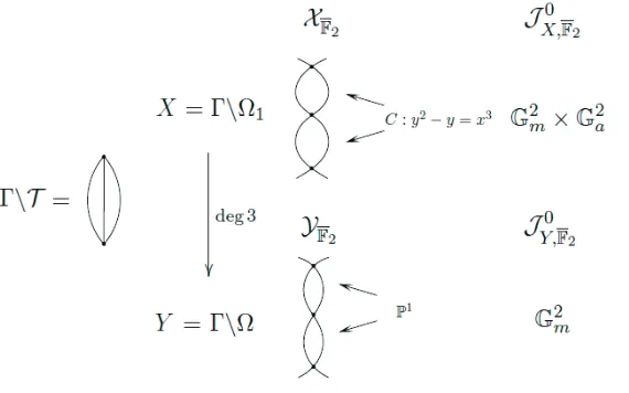
half-plane Ω. We use the covering to describe the geometry of X mod pand compute the Néron modelJX ofJX overZp. LetY be the Shimura curve with the same tame level (i.e.,

the level away fromp) asX but with the level atpreplaced byO×p. ThenX→Y is a finite

cover of degreep+ 1.

Theorem 1.13 (Theorem 5.16). LetJX (resp. JY) be the Néron model of JX (resp. JY)

overZp. Suppose the tame level is small enough. Then the identity component of the special

fiber of the Néron models are given by

(19)

1.6. Level raising and rank lowering

respectively. HereT is a torus of dimension equal to the genusg(Y) ofY andU is a vector group (i.e., a product ofGa’s) of dimension g(X)−g(Y).

Remark 1.14. We will further determine their component groups in Theorem 5.16 (3).

Remark 1.15. For the Shimura curve Y with maximal level at p, its Néron model JY has

been computed by Jordan–Livné [JL86]. Our contribution is the determination of JX for

the Shimura curve X with deeper, but still in some sense, “tame” level at p. The two key ingredients are Teitelbaum’s theorem [Tei90] on the rigid geometry of Ω1 and Edixhoven’s

theorem [Edi92] on the behavior of Néron models under tamely ramified extensions.

1.6 Level raising and rank lowering

In the last Chapter 6, we follow the ingenious strategy of W. Zhang for proving the p-indivisibility Conjecture 1.9 whenp≥5 and investigate the relevant problems forp= 2.

Suppose we are in the situation of Conjecture 1.9. This strategy reduces the problem in rank one to rank zero via level raising, roughly consists of three steps:

A: Letf ∈S2(N)be the newform associated toE/Q. Find a congruencef ≡g (modp)

betweenf and another newformg∈S2(N q)with level raised at some prime q.

B: LetA=Agbe the elliptic curve associated tog(whengdoes not have rational Fourier

coefficients, one works with the corresponding modular abelian variety instead). Prove that one can always findg in Step A such thatq is inert inK and sp(A/K) = 0.

C: Show that

yK 6∈pE(Kq)⇐⇒sp(A/K) = 0.

Step A is ensured by the level raising theorem of Ribet ([Rib90]) for anyp.

(20)

1.7. Obstruction for rank lowering

Step C can be thought of as a congruence between (suitably defined algebraic parts of)

L′_(E/K) _and _L(A/K)_:

• the p-part of L′_(E/K) _{is related to the} _p_{-divisibility of Heegner points} _y

K by the

Gross-Zagier formula;

• thep-part of L(A/K) is related tosp(A/K)by BSD.

Its proof combines the Jochnowitz congruence established by Bertolini–Darmon [BD99] for

p≥5, Gross’ explicit Waldspurger formula [Gro87], and the p-part of BSD formula in the caseran= 0due to Skinner–Urban forp≥3.

We can depict the three steps as follows.

E

A B: Rank lowering

f ≡≡

g

O

(modp) A: Level raising

L′_{(f /K,}₁₎ _“_≡≡_” _L(g/K,₁₎ _(mod_p) _{C: Jochnowitz congruence}

1.7 Obstruction for rank lowering

Now we specialize the previous section to the casep= 2. Letρ¯= ¯ρE,2 :GQ→Aut(E[2])∼=

GL2(F2) be the Galois representation on the 2-torsion points. The level raising theorem

(Step A) in this case asserts thatq ∤2N is a level raising prime if and only ifρ(Frob¯ q) = (1 00 1)

or (1 1

0 1). Under Assumption 6.1 and 6.13, we prove a parity conjecture on 2-Selmer ranks

(21)

1.7. Obstruction for rank lowering

Theorem 1.16 (Theorem 6.27). Suppose ρ(Frob¯ q) = (1 10 1). Then

s2(E/K) =s2(A/K)±1.

It follows that ifs2(E/K) = 1, thens2(A/K) = 0or2. However, the Chebotarev density

argument (in Step B) fails and does not show that one can always get s2(A/K) = 0. In

fact, we prove the following surprising obstruction for rank lowering: whenρ(Frob¯ q) = (1 1_{0 1}),

s2(A/K)can never be lowered to zero!

Theorem 1.17 (Theorem 6.29). Suppose ρ(Frob¯ q) = (1 1_{0 1}). Then

s2(E/K) = 1 =⇒s2(A/K) = 2.

Remark 1.18. Theorem 1.17 tells us that Step B of the strategy cannot naively work for

p= 2. In joint work with B. Le Hung [LL15], we enhance Ribet’s level raising theorem to raise the level at multiple primes simultaneously, using the method of [DT94] and [All14].

With a refined control over the signs (which are not detected under the mod 2 congruence),

we show that it is possible to obtainarbitrary s2(A/Q)via level raising mod 2. In particular,

there is no obstruction for rank lowering over Q in contrast to the situation over K. The

spirit of this result is similar to the work of Mazur–Rubin [MR10] on arbitrary 2-Selmer

ranks in quadratic twist families. This obstruction for rank lowering is a phenomenon unique

(22)

Chapter 2 2-Selmer groups and 2-class groups

Let E/Q be an elliptic curve. We will impose the following assumptions throughout this chapter.

Assumption 2.1. SupposeE has equationy2 ₌_F_(x)_{, where}_F_{(x) =}_x3₊_a

2x2+a4x+a6

is an integral polynomial which (1) is irreducible, and

(2) has negative and square-free discriminant−D.

LetL=Q[x]/F(x). Then Lhas the following elementary properties:

(1) SinceF(x)is irreducible and has negative discriminant, we know thatF(x)has Galois groupS3. The fieldL=Q[x]/F(x)is a complex cubic field, i.e.,L∞:=L⊗QR∼=R×C.

(2) SincediscF(x) =−Dis square-free, we know thatD≡3 (mod 4),Lhas discriminant

dL = discF(x) =−D, andLhas ring of integersA=Z[x]/F(x).

(3) SinceLhas a unique real embedding, we know that the unit group A× has rank one by Dirichlet’s unit theorem. LetuL be a fundamental unit. Then A× =uZ_L× {±1}.

After possibly replacinguL by−uL, we may assumeuL >0. After possibly replacing

(23)

2.1.

The elliptic curveE:y2 ₌_F_(x) _{has the following elementary properties:}

(1) SinceF(x)is irreducible, we haveE(Q)[2] = 0.

(2) The 2-torsion fieldQ(E[2]), as the Galois closure ofL, is an S3-extension over Q.

(3) E has discriminant ∆ = −24D. Since no 12th power divides ∆, the equation y2 = F(x) is minimal. It follows thatE has bad reduction precisely atp|2D.

(4) Forp|D, sinceDis square-free, by comparing the power ofpappearing on both sides of

c3₄−c2₆ =−210·33·D,

we see that p ∤ c4. Hence E has multiplicative reduction of type I1 at p | D. In

particular, the component group of the Néron model ofE/Qp is trivial.

(5) We compute thatc4 = 16(a22−3a4), so2|c4 and E has additive reduction at 2.

(6) Therefore the conductor ofEis of the formN = 22+δD for some δ≥0. The order of

N at 2 is determined by the Ogg–Saito formula ([Sil94, 11.1])

ord2(N) = ord2(∆) + 1−m= 5−m, (2.1)

wherem is the size of the component group of the Néron model ofE/Q2.

(24)

2.1. 2-Selmer groups

2.1 2-Selmer groups

Recall that for an elliptic curveE/Q, we have the global and local Kummer exact sequences, fitting into the following commutative diagram

0 //_E(_Q_)/2E(_Q₎ δ //

H1(Q, E[2]) // Q

vresv

H1(Q, E)[2] //

0

0 //Y

v

E(Qv)/2E(Qv)

Q

vδv

/

/Y

v

H1(Qv, E[2]) //

Y

v

H1(Qv, E)[2] //0.

Here the vertical maps are given by the product of restriction maps over all placesv ofQ.

Definition 2.2. The 2-Selmer group

Sel2(E/Q)⊆H1(Q, E[2])

consists of cohomology classes whose restriction atvlies in the image of the local Kummer mapδv for everyv:

Sel2(E/Q) ={c∈H1(Q, E[2]) : resv(c)∈im(δv)}.

Colloquially, the 2-Selmer group is cut out by thelocal conditions

im(δv)⊆H1(Qv, E[2])

coming from local points for allv. By definition, we have an injection

E(Q)/2E(Q)֒→Sel2(E/Q).

(25)

2.2. Kummer maps

s2(E/Q) := dimF2Sel2(E/Q)provides an upper bound for the rank of E(Q).

2.2 Kummer maps

Our first goal is to give an explicit description of the global and local Kummer maps in terms of the cubic fieldL.

Lemma 2.3. We have an exact sequence of finite group schemes over Q,

1→E[2]→Res_L/_Qµ2−→N µ2→1,

where N is induced by the norm map fromL to Q. We have an isomorphism

H1(Q, E[2])∼= (L×/(L×)2)N=✷. (2.2)

Here (L×/(L×)2)N=✷ consists of all classes inL×/(L×)2 with square norms to Q×.

Proof. It suffices to check that we have an exact sequence of GQ-modules on the level of

Q-points. Suppose F(x) has the three roots x1, x2, x3 ∈ Q. Then the Q-points of E[2]

consist of Pi = (xi,0), (i = 1,2,3) and ∞. The Galois group GQ acts trivially on ∞and permutes the three pointsPi via itsGal(Q(E[2])/Q)∼=S3-action on xi. Also, the group of

Q-points ofRes_L/_Qµ2 is isomorphic toµ2×µ2×µ2, where the three factors are indexed by

the three rootsxi and the Galois action permutes the three factors in the same way. The

norm map simply multiplies the three factors and respects the GQ-action. One sees that

the map

∞ 7→(1,1,1), P17→(1,−1,−1), P27→(−1,1,−1), P3 7→(−1,−1,1)

gives an injective homomorphism of GQ-modulesE[2]→ResL/Qµ2. Moreover, its image is

(26)

2.2. Kummer maps

Taking the long exact sequence in Galois cohomology, we obtain

H0(Q,ResL/Qµ2)−→N H0(Q, µ2)→H1(Q, E[2])→H1(Q,ResL/Qµ2)−→N H1(Q, µ2).

Since H0(Q,ResL/Qµ2) = µ2(L) = {±1}, H0(Q, µ2) = µ2(Q) = {±1} and L/Q has odd

degree, we know that the first map is surjective. By Kummer theory, we know that

H1(Q,ResL/Qµ2)∼=L×/(L×)2, H1(Q, µ2)=∼Q×/(Q×)2.

Therefore

H1(Q, E[2]) = ker(N:L×/(L×)2→Q×/(Q×)2) = (L×/(L×)2)N=✷.

This finishes the proof of the second part.

Proposition 2.4. Under the isomorphism (2.2), the global Kummer mapδ can be described as

δ:E(Q)/2E(Q)→(L×/(L×)2)N=✷, P 7→x(P)−β,

where x(P) is thex-coordinate of P and β is the image of x inL=Q[x]/F(x).

Proof. Lete2:E[2]×E[2]→µ2 be the Weil pairing. Then we see that the homomorphism

E[2]→Res_L/_Qµ2 in Lemma 2.3 is also given by

P 7→(e2(P, P1), e2(P, P2), e2(P, P3)).

The rational function fi = x−xi has the divisor (fi) = 2Pi−2∞ (i = 1,2,3) and there

exists some rational functiongi(overQ) such thatfi◦[2] =g2_i (see [Sil09, III.8]). The Weil

pairing e2 is then given by

e2(P, Pi) = gi(X+P)

(27)

2.2. Kummer maps

where X∈E(Q)is any point such that g(X+P)and g(X)are both defined and nonzero. For P ∈ E(Q), we choose Q ∈E(Q) such that[2]Q = P. Then δ(P) corresponds to the cocycle{σ7→Qσ−Q} ∈H1(Q, E[2]). TakingP =Qσ−QandX =Q, we know that

e2(Qσ−Q, Pi) = gi(Q) σ

gi(Q) . (2.3)

By the identification H1(Q,ResL/Qµ2) ∼= (L×/(L×)2)N=✷ coming from Kummer theory,

Equation (2.3) implies that

δ(P)≡gi(Q)2 mod (L×)2

under the embedding L ֒→ Q associated to xi. But by the construction of gi, we have

gi(Q)2 =fi(P) =x(P)−xi. Hence

δ(P)≡x(P)−xi mod (L×)2

under the embeddingL ֒→Q associated to xi, which finishes the proof.

Base changing toQvin Lemma 2.3 and Proposition 2.4 , we obtain the analogous explicit

description of the local Kummer maps δv.

Proposition 2.5. The local Kummer maps for E are given by

δv :E(Qv)/2E(Qv)→H1(Qv, E[2])= (L∼ ×v/(L×v)2)N=✷, P 7→x(P)−β,

where β is the image of xin Lv=Qv[x]/F(x).

Remark 2.6. Even though E(Q)[2] = 0, it is possible that E(Qv)[2] 6= 0. For a nonzero

pointP ∈E(Qv)[2], the expressionx(P)−βdoes not lie inL×v and it should be interpreted

(28)

2.3. Local conditions

which are not 2-torsion, thenδv(P) = (x(P1)−β)/(x(P2)−β).

2.3 Local conditions

Our next goal is to describe explicitly the local conditionim(δv)for each placev.

Lemma 2.7. Let p be a prime. Then the valuation of δp(P) is even for any P ∈E(Qp),

namely,

δp(P)∈(A×p/(A×p)2)N=✷,

where A=Z[x]/F(x) is the ring of integers ofLand Ap=A⊗Zp.

Proof. Let P ∈E(Qp)and writex=x(P) for short.

First consider the casep∤D. So pis unramified in L. There are three cases:

(1) Lp ∼= Qp3 is the unramified cubic extension of Q_p. From y2 = F(x), we know that 2 ordp(y) = 3 ordp(x−β), henceordp(x−β)is even.

(2) Lp ∼= Qp2 ×Q_p, where Q_p2 is the unramified quadratic extension of Q_p. Write β = (γ, c), then γ 6≡c (modp), ordp(γ) = 0and ordp(c) ≥0. Fromy2 =F(x), we know

that2 ordp(y) = ordp(x−γ) + ordp(x−c). There are two cases:

• Ifordp(x)<0, thenordp(x−γ) = ordp(x−c) = ordp(x). Therefore2 ordp(y) =

3 ordp(x), henceordp(x−γ) = ordp(x−c) = ordp(x)are all even.

• Ifordp(x)≥0, then ordp(x−γ) = 0. Soordp(x−c) = 2 ordp(y) is even.

(3) Lp ∼= Qp×Qp×Qp. Write β = (c1, c2, c3). Then ci 6≡ cj (modp) whenever i 6= j.

Similarly, there are two cases:

• If ordp(x) < 0, then ordp(x−ci) = ordp(x). Therefore 2 ordp(y) = 3 ordp(x),

(29)

• Ifordp(x)≥0, then ordp(x−ci)≥0. Sinceci6≡cj (modp), at least two of the

ordp(x−ci)’s are zeros. Thus2 ordp(y) = ordp(x−c1)+ordp(x−c2)+ordp(x−c3)

implies the third one must have even valuation as well.

Now consider the casep|D. Sopis ramified inL. SinceDis square-free, we know that

Lp ∼= Kp×Qp, where Kp is a ramified quadratic extension of Qp. Denote by p the prime

for Kp and write β = (γ, c). Then γ 6≡ c (modp), ordp(γ) > 0 and ordp(c) ≥ 0. From

y2 =F(x), we know that 2 ordp(y) = ordp(x−γ) + ordp(x−c). We argue similarly:

• Ifordp(x)<0, thenordp(x−γ) = 2 ordp(x)andordp(x−c) = ordp(x). Henceordp(x)

is even, therefore bothordp(x−γ) andordp(x−c)are even.

• Ifordp(x) ≥ 0, then ordp(x−γ) ≥ 0 and ordp(x−c) ≥0. Since γ 6≡ c (modp), at

least one ofordp(x−γ) andordp(x−c)is zero. Hence both of them are even.

Remark 2.8. When p6= 2, Lemma 2.7 can be proved by a more “pure thought” argument: since the component group of Néron model of E/Qp is trivial, the local condition at p

corresponds to the unramified cohomologyH_ur1(Qp, E[2])([GP12, Lemma 6]), which consists

of the units (A×_p/(A×_p)2)N=✷ under the isomorphism (2.2). Here we preferred the above

direct computational proof using the explicit description of δp in Proposition 2.5, which

depends on less machinery and also treats the casep= 2.

Proposition 2.9. We have

(1) Forv=∞, bothE(R)/2E(R)and(L×_∞/(L×_∞)2)N=✷ are trivial. In particular, the local condition im(δ∞) is trivial.

(2) Forv=p >2, the local conditionim(δp) = (A×p/(A×p)2)N=✷.

(30)

Proof. For v=∞, since L∞ ∼=R×C, we know that

(L×_∞/(L×_∞)2)N=✷= (R×/(R×)2)N=✷={1}.

For v = p, we know from Lemma 2.7 that im(δp) ⊆ (Ap×/(A×p)2)N=✷. Since the norm

map is surjective on the units, we know that

#(A×_p/(A×_p)2)N=✷= #A×

p/(A×p)2

#Z×p/(Z×p)2

.

Notice that#Z×

p/(Z×p)2is22 or2depending on whether p= 2or not. IfLp is a product of

k fields (k = 1,2,3), then #A×

p/(A×p)2 is2k+3or 2k depending on whetherp= 2or not. It

follows that

#(A×_p/(A×_p)2)N=✷=       

2k−1, p6= 2, 2k+1, p= 2.

SinceE(Qp) has a finite index subgroup isomorphic toZp, we know that

#E(Qp)/2E(Qp) =

      

#E(Qp)[2], p6= 2,

2·#E(Qp)[2], p= 2.

All claims except the last one then follow because #E(Qp)[2] is the same as 1 plus the

number of Qp-rational solutions of F(x) = 0 , which is 2k−1 in all cases. To see the last

claim thatim(δ2) contains all the units ≡1 (mod 4), let us consider a point P ∈E(2ˆ Z2),

where Eˆ is the formal group of E over Q2 given by the minimal equation. For a general

elliptic curveE with minimal equation

(31)

2.4. 2-class groups of cubic fields

the general formula ([Sil94, IV.1]) reads

x(P) =z−2−a1z−1−a2−a3z+O(z2),

where z=−x/y is the parameter for the formal group. In our casea1= 0, therefore

δ2(P) =x(P)−β=z−2−a2−β+O(z)≡1−(a2+β)z2+O(z3)≡1−(a2+β)z2 mod (L×2)2,

(2.4) where the last equality is because z ∈ 2Z2 and the units ≡ 1 (mod 8) are squares. Since

F(x) mod 2 cannot be a product of three distinct linear factors in F2[x], we know that 2

does not split in L. Now one can then check directly that im(δ2) contains the units ≡ 1

(mod 4)with square norm in the remaining two cases:

• IfL2 = Q8, then all units ≡ 1 (mod 4) with square norms are actually squares. So

the claim thatim(σ2) contains all such units is trivial.

• IfL2= Q4×Q2, then any class (α, a)≡1 (mod 4) with square norm is represented

by (α,Nα) with α ≡ 1 (mod 4). There is a unique nontrivial class of units α ≡ 1 (mod 4)modulo squares, represented by1 + 4γ if we writeβ = (γ, c). It follows from (2.4) thatim(δ2)contains this class.

2.4 2-class groups of cubic fields

Combining all the local conditions gives us both upper and lower bounds for the 2-Selmer group.

Lemma 2.10. Let

(32)

and

M2 ={α∈L×/(L×)2:α >0,(α) =I2, I ⊆La fractional ideal}

be subgroups of (L×_/(L×₎2₎

N=✷. Then under the isomorphism (2.2), we have

M1 ⊆Sel2(E/Q)⊆M2.

Proof. Elements ofM2clearly have square norms sinceNα=N(I)2. Ifα∈Sel2(E/Q), then

by Proposition 2.9, α >0 and α has even valuation at all finite places. The latter implies that there exists a fractional idealI such that(α) =I2. Thus α∈M2.

Let α ∈ L×/(L×)2. For p odd, Lp(√α)/Lp is unramified if and only if α has even

valuation. For p = 2, L2(√α)/L2 is unramified if and only if α has even valuation and

is represented by a unit ≡ 1 (mod 4). From this description we see that M1 ⊆ M2 and

elements M1 have square norm. It also follows from this description and Proposition 2.9

thatM1⊆Sel2(E/Q).

Class field theory supplies information about the two groupsM1 andM2.

Lemma 2.11. Let Cl(L) be the ideal class group of the cubic field L = Q[x]/F(x). Let k= dimF2Cl(L)[2]. ThenM1 (resp. M2) is an elementary 2-group of size2k (resp. 2k+1).

Proof. Kummer theory tells us that

M1∼= Hom(Gal(M/L), µ2),

whereM is obtained by adjoining the square roots of allα∈M1toL, which is the maximal

unramified extension ofLof exponent 2. By class field theory, we have

Gal(M/L)∼= Cl(L)[2].

(33)

Supposeα ∈M2 such that (α) =I2. Then the assignment α7→I gives a well defined

map

M2→Cl(L)[2].

This map is clearly surjective and its kernel is given by the positive units

{α∈A×/(A×)2 :α >0}=uZ_L/u2_LZ∼=Z/2Z.

Since# Cl(L)[2] = 2k, we know thatM2 is an elementary 2-group of size 2k+1.

Now we are ready to prove the main theorem of this chapter.

Theorem 2.12. Let Cl(L) be the ideal class group of the cubic field L= Q[x]/F(x). Let k= dimF2Cl(L)/2 Cl(L). Then

s2(E/Q) =k or k+ 1,

depending on whether the root number ε(E/Q) = (−1)k or (−1)k+1. In particular, if the class numberhL of Lis odd (i.e., k= 0), then

s2(E/Q) = 0 or1,

depending on whether ε(E/Q) = +1 or−1.

Proof. It follows from Lemma 2.10 and 2.11 that s2(E/Q) = k or k + 1. By [Mon96,

Theorem 1.5], the parity ofs2(E/Q) is determined by the root numberε(E/Q), that is,

(−1)s2(E/Q)

=ε(E/Q).

(34)

Chapter 3 Artin

L

-functions

In this chapter, we explain how Theorem 2.12, under the BSD conjecture, can be interpreted as a mod 2 congruence between the weight 2 newformf ∈S2(N) associated toE/Qand a

weight 1 newformhassociated to a certain 2-dimensional Artin representation σ.

Let E/Q be an elliptic curve. Letρ¯: GQ →Aut(E[2]) ∼= GL2(F2) =S3 be its mod 2

Galois representation. We will impose the following assumptions throughout this chapter.

Assumption 3.1.

(1) ρ¯is surjective.

(2) E has negative discriminant∆.

Remark 3.2. ρ¯is surjective if and only if the 2-torsion fieldQ(E[2])is an S3-extension over Q. When E:y2₌_F_(x)_{is defined by a cubic polynomial}_F_(x)_∈_Q_[x]_{, this happens if and}

(35)

3.1. Artin representations and class numbers

3.1 Artin representations and class numbers

Definition 3.3. LetV be the unique 2-dimensional complex representation of GL2(F2) =

S3. We define a complex representationσ to be the composition

σ:GQ−→ρ¯ GL2(F2)→GL(V)∼= GL2(C).

The kernel ofσ cuts out the S3-extensionQ(E[2])/Q, the Galois closure of the cubic field

L=Q[x]/F(x). We writeG= Gal(Q(E[2])/Q)∼=S3 for short.

Let L(σ, s) be the Artin L-function of σ (for background on Artin L-functions, see [Tat11]). It has holomorphic continuation toC and satisfies a functional equation relating its values atsand1−s. Sinceσis self-dual of orthogonal type (its image can be conjugated intoO2(R)), the sign of its functional equation is always+1 ([FQ73]). More precisely, let

Λ(σ, s) = ((2π)−sΓ(s))dimσL(σ, s)

be the complete L-function, then

Λ(σ, s) =N(σ)1/2−sΛ(σ,1−s),

whereN(σ)is the Artin conductor ofσ, a positive integer measuring the ramification ofσ.

Proposition 3.4. Let ζQ(s) be the Riemann zeta function and ζL(s) be the Dedekind zeta

function of the cubic fieldL. Then

ζQ(s)·L(σ, s) =ζL(s).

In particular,

(36)

3.2. The determinant and conductor

where dL is the discriminant ofL.

Proof. Let H ⊆ G ∼= S3 be a subgroup of order two. Then L ∼= Q(E[2])H. From the

basic property of the ArtinL-function of an induced representation, we know thatζL(s) =

L(IndG_H1H, s). Since IndGH1H = 1G⊕σ, we haveζL(s) = L(1G, s)L(σ, s) =ζQ(s)L(σ, s).

The claim thatN(σ) =dL then follows from the conductor-discriminant formula.

Corollary 3.5. L(σ, s) has a simple zero ats= 0and

L(σ,1) = 2π hLloguL |dL|1/2

, L′(σ,0) =hLloguL.

Here uL>1 is a fundamental unit ofL.

Proof. By the class number formula, for any number field K, ζK(s) has a simple pole at

s= 1with residue 2r1(2π)r2hKRK

wK|dK|1/2 and has a zero of orderr1+r2−1with leading coefficient

−hKRK

wK . In particular,

(1) ζQ(s) has a simple pole ats= 1with residue 1 and has value ζQ(0) =−1₂; (2) ζL(s) has a simple pole at s = 1 with residue 2πh_|_dLloguL

L|1/2 and a simple zero at s = 0

with leading coefficient−hLloguL

2 .

The corollary then follows from Proposition 3.4.

3.2 The determinant and conductor

Proposition 3.6. detσ = εK, where εK is the quadratic character associated to K =

Q(√∆). In particular, σ is an odd irreducible Artin representation.

Proof. Since σ has S3-image, it is induced from a cubic characterχ:GK →C×, where K

is the quadratic field corresponding to the sign representation

(37)

The unique quadratic subfield of Q(E[2]) is K = Q(√∆), where ∆ is the discriminant of

E/Q([Ser72, p. 305]). By the general formula for the determinant of an induced represen-tation, we have

detσ= det(IndGQ

GKχ) =ǫK ·χQ,

where χQ :GabQ

Ver

−−→Gab

K χ

−→C×_{is the transfer of}_χ_{. Since} _Gab _{= Gal(K/}_Q₎_{, it follows that}

χQ is trivial. Since we assumed that ∆<0, we know that K is imaginary anddetσ= εK

is−1on the class of complex conjugation, i.e., σ is odd.

By the general conductor formula for induced representations, we also have

Proposition 3.7. N(σ) =|dK| ·N(χ), where N(χ)is the Artin conductor of χ.

We now further determine the Artin conductor N(σ) in terms of the Serre conductor

N(¯ρ)of the mod 2 representation ρ¯.

Proposition 3.8. We haveN(σ) =N(¯ρ), 4N(¯ρ), or 8N(¯ρ). Moreover,

(1) IfE has good supersingular reduction at 2, thenN(σ) = 4N(¯ρ).

(2) If E has good ordinary reduction at 2, then N(σ) = N(¯ρ) or 4N(¯ρ) depending on whether 2 is unramified inK =Q(√∆) or not.

(3) IfE has multiplicative reduction at 2, then the even part of N(σ) is equal to the even

part ofdK.

(4) IfE has additive reduction at 2 and satisfies Assumption 2.1, thenN(σ) =N(¯ρ) =D.

Proof. By definition, the odd parts of N(σ)and N(¯ρ)coincide and it remains to determine the even part ofN(σ). LetD⊆G∼=S3be the decomposition group at 2 and I✁D be the

inertia subgroup at 2. We have following cases:

(38)

(2) IfDis of order 2, thenI is either trivial or of order 2. (3) IfDtrivial, then I is trivial.

We can determine the even part ofN(σ)depending onI: (1) IfI is trivial, thenσ is unramified at 2 and N(σ) =N(¯ρ).

(2) IfI is of order 3, thenσ is tamely ramified at 2,VI _{= 0}_{and hence}_N_{(σ) = 4N}_(¯_ρ)_.

(3) IfI is of order 2, then the even part ofN(σ) =|dL| (by Proposition 3.4) is equal to

the discriminant of a ramified quadratic extension ofQ2, which is either 4 or 8, hence

N(σ) = 4N(¯ρ) or8N(¯ρ).

(4) WhenI is trivial or of order 2, the even part ofN(σ) =dL is equal to the even part

ofdK. Moreover,I is of order 2 if and only if 2 is ramified inK=Q(

√ ∆). Now we can conclude:

(1) If E has good supersingular reduction at 2, then σ|D is irreducible ([Ser72, p.275,

Prop.12]), henceI is of order 3 andN(σ) = 4N(¯ρ).

(2) IfEhas good ordinary reduction at 2, then the image ofσ|D is contained in the Borel

subgroup of GL2(F2), which has order 2. Hence I is either trivial or order 2. Since

E has good reduction at 2, we know that 2 ∤ ∆, hence the 2-part of dK is 0 or 4,

depending whether 2 is ramified inK or not.

(3) IfE has multiplicative reduction at 2, then the image ofσ|D is also contained in the

Borel subgroup ofGL2(F2), which has order 2. HenceI is either trivial or order 2.

(4) IfE has additive reduction at 2 and satisfies Assumption 2.1, we have dL = −D is

(39)

3.3. Weight one newforms

3.3 Weight one newforms

Write L(σ, s) =P

n≥1bnn−s. Then bp = Tr(σ(Frobp)) for any p ∤ N(σ). In particular, bp

takes values2,0,−1whenFrobp∈G∼=S3is of order1,2,3respectively. The determination

ofdetσandN(σ)in Proposition 3.6 and 3.8 is even more interesting in view of the following

Theorem 3.9. The formal series h(z) = P

n≥1bnqn is the q-expansion of a weight one

newform of level N(σ) and nebentypus detσ=εK.

Proof. This is a special case of Langlands–Weil for 2-dimensional odd irreducible Artin representations with solvable image (see [Ser77, Theorem 1]). The construction in our dihedral case was due to Hecke. Let ψ : A×_K → C× be the Hecke character associated to the cubic character χ: GK →C× (recall thatσ = IndG_GQ_Kχ). Then the Hecke theta series

associated to ψ,

˜

h(z) := X

a⊆OK

ψ(a)qNa,

where the sum runs over all integral ideals, is a weight one newform with nebentypus εK

and level |dK| ·N(ψ), which is equal to N(σ) by Proposition 3.7 (see [Miy89, 4.8.2] for a

proof using Weil’s converse theorem). Let ˜bp be the p-th Fourier coefficient of ˜h(z), then

˜_b_p₌P

Np=pψ(p). We easily see that for p∤N(σ),

˜_b_p ₌               

2, if p=ppis split in K, ψ(p) = 1,

0, if pis inert inK,

−1, if p=ppis split in K, ψ(p) =a primitive 3rd root of unity.

By class field theory, the three cases exactly correspond to Frobp∈G∼=S3 having order 1,

2 and 3. It follows that ˜bp = Tr(σ(Frobp)) = bp forp ∤ N(σ) and thus ˜h(z) = h(z) is the

(40)

3.3. Weight one newforms

Corollary 3.10. Let f = P

n≥1anqn ∈ S2(N) be the weight 2 newform of level N and

trivial nebentypus associated to the elliptic curveE. Then for any prime p6= 2,

ap≡bp (mod 2).

Moreover, we can determine the parity of a2 andb2 as follows.

(1) IfE has good supersingular reduction at 2, thena2≡0 (mod 2),b2= 0.

(2) If E has good ordinary reduction at 2, then a2 ≡ 1 (mod 2). In this case, if 2 is

ramified in K, then b2= 1; otherwiseb2 = 0or2.

(3) If E has multiplicative reduction at 2, then a2 =±1. In this case, if 2 is ramified in

K, then b2= 1; otherwiseb2= 0 or2.

(4) IfE has additive reduction and satisfies Assumption 2.1, then a2= 0. In this case, if

2is inert in the cubic field L, thenb2 =−1; otherwiseb2= 0.

Proof. The mod 2 congruence follows by construction. All claims about a2 are also clear.

To prove the claims about b2 = Tr(σ(Frob2)|VI), whereI is the inertia subgroup at 2, we

proceed case by case as in the proof of Proposition 3.8.

(1) IfE has good supersingular reduction, thenI has order 3. HenceVI = 0and b2 = 0.

(2) If E has good ordinary or multiplicative reduction. Then I is either of order 2 or trivial, depending on whether 2 is ramified in K or not. If I is order 2, then VI

is 1-dimensional and the action of Frob2 is trivial, thus b2 = 1. If I is trivial, then

VI =V and the action ofFrob2 is either of order 2 or trivial, thusb2 = 0or2.

(3) IfEhas additive reduction and satisfies Assumption 2.1, thenI is trivial andVI =V. SinceF(x) mod 2cannot be a product of three distinct linear factors inF2[x], we know that 2 does not split inL. If 2 is inert in L, then Frob2 is of order 3 and b2 = −1;

(41)

3.4. Examples

To summarize, we obtain a congruence between a weight two newform and a weight one newform

f ≡h (mod 2),

in the sense that all (except possibly for p = 2) of their Hecke eigenvalues are congruent mod 2. As explained in the introduction, under the BSD conjecture, Theorem 2.12 can be interpreted as a mod 2 congruence between the special values of the L-functionsL(f, s) = L(E, s) andL(h, s) =L(σ, s).

Remark 3.11. We find this mod 2 congruence rather unusual: L(E, s)is of symplectic type with the sign of the functional equation ±1 whereas the Artin L-function L(σ, s) is of orthogonal type with the sign of the functional equation always +1. Congruences of this type mod p > 2 would force the signs to be the same. As Mazur pointed out to us, this may suggest something much more general with intersections mod 2 of 2-adic eigenvarieties

of different (symplectic versus orthogonal) reductive groups.

Also, the points= 1is the central critical point forL(E, s)but there is no critical point for L(σ, s) in the sense of Deligne. We hope to formulate this type of mod 2 congruence

betweenL-functions more precisely in the future.

3.4 Examples

We end our discussion on 2-Selmer groups and class numbers with several explicit examples.

Example 3.12 (cf. [Ser77, 7.3]). Consider the elliptic curve

E= 92a1 :y2 =F(x) =x3+x2+ 2x+ 1.

The polynomialF(x)is irreducible and has square-free and negative discriminant−D=−23

(42)

3.4. Examples

conductorN = 22_·₂₃_{. The cubic field}

L=Q[x]/(x3+x2+ 2x+ 1)

has discriminant dL = −23, hence the Artin representation σ has conductor N(σ) = 23.

The class number ofLis 1 and we have s2(E/Q) = 0 as predicted by Theorem 2.12.

Notice thatdK =−23, soN(χ) = 1by Proposition 3.7, i.e.,χis unramified. Hence the

Hecke characterψcan be viewed as an order 3 character on the ideal class groupCl(K). We remark thatKis the cubic field ofsmallest (in the sense of the absolute value) discriminant with class number 3. The three ideal classes inCl(K)are represented by the three integral binary quadratic forms of discriminantdK =−23,

x2+xy+ 6y2, 2x2±xy+ 3y2,

of order 1 and 3 respectively. We find thath(z) is the following simple linear combination of theta series associated to these quadratic forms:

h(z) = 1 2



 X

m,n∈Z

qm2+mn+6n2− X

m,n∈Z

q2m2+mn+3n2 



=q−q2−q3+q6+q8−q13−q16+q23−q24+q25

+q26+q27−q29−q31+q39−q41−q46−q47+q48+q49−q50· · ·

We remark thatσis the irreducible 2-dimensional Artin representation ofsmallestconductor ([Ser77, 8.1]). Moreover,h(z) can be written as the classical eta product:

h(z) =η(z)η(23z) =qY

n≥1

(43)

3.4. Examples

where

η(z) =q1/24Y

n≥1

(1−qn) =X

n≥1

12

n

qn 2 24

is Dedekind’s eta function.

The first few Hecke eigenvalues of the newformsf(z)∈S2(92) and h(z)∈S1(23, ε−23)

are listed in Table 3.1. We see that ap ≡bp (mod 2) for p6= 2, a2 = 0and b2 = −1 as in

Corollary 3.10 (2 is inert in L).

p 2 3 5 7 11 13 17 19 23 29 31 37 41 43 47

ap(f) 0 1 0 2 0 −1 −6 2 −1 −3 5 8 3 8 9

bp(h) −1 −1 0 0 0 −1 0 0 1 −1 −1 0 −1 0 −1

Table 3.1: E = 92a1

Example 3.13. Consider elliptic curve

E =X0(11) = 11a1 :y2+y=x3−x2−10x−20,

which has the smallest conductor 11 among all elliptic curves overQ. It has discriminant

∆ =−11and has good supersingular reduction at 2. The cubic field

L∼=Q[x]/(x3−x2+x+ 1)

has discriminant dL = −22·11. Hence the Artin representation σ has conductor N(σ) =

22·11. The class number ofLis 1 and we haves2(E/Q) = 0as predicted by Theorem 2.12.

The ring class group of the quadratic order of discriminant −44 in K= Q(√−11) has order 3, represented by the three binary quadratic form of discriminant−44,

2x2+ 11y2, 3x2±2xy+ 4y2

(44)

3.4. Examples

of theta series associated to these quadratic forms:

h(z) = 1 2



 X

m,n∈Z

q2m2+11n2 − X

m,n∈Z

q3m2+2mn+4n2 



=q−q3−q5+q11+q15−q23+q27−q31−q33−q37+ 2q47+q49+· · ·

Moreover,h(z) is the classical eta product

h(z) =η(2z)η(22z) =qY

n≥1

(1−q2n)(1−q22n).

The newformf(z)∈S2(11) is also a classical eta product

f(z) =η2(z)η2(11z) =qY

n≥1

(1−qn)2(1−q11n)2

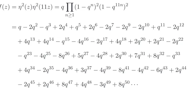
=q−2q2−q3+ 2q4+q5+ 2q6−2q7−2q9−2q10+q11−2q12 + 4q13+ 4q14−q15−4q16−2q17+ 4q18+ 2q20+ 2q21−2q22 −q23−4q25−8q26+ 5q27−4q28+ 2q30+ 7q31+ 8q32−q33 + 4q34−2q35−4q36+ 3q37−4q39−8q41−4q42−6q43+ 2q44 −2q45+ 2q46+ 8q47+ 4q48−3q49+ 8q50· · ·

The first few Hecke eigenvalues of the newformsf(z)∈S2(11) and h(z)∈S1(44, ε−44)

are listed in Table 3.2. We see thatap≡bp (mod 2)for allpas in Corollary 3.10.

p 2 3 5 7 11 13 17 19 23 29 31 37 41 43 47

ap(f) −2 −1 1 −2 1 4 −2 0 −1 0 7 3 −8 −6 8

[image:44.595.140.462.392.544.2]

bp(h) 0 −1 −1 0 1 0 0 0 −1 0 −1 −1 0 0 2

(45)

3.4. Examples

Example 3.14. Consider the elliptic curve

E = 26a1 :y2+xy+y=x3−5x−8.

It has discriminant∆ =−23·133 and has nonsplit multiplicative reduction at 2. The cubic field

L∼=Q[x]/(x3−x−2)

has discriminant dL = −23 ·13 = −104. Notice that dK = −23· 13, so N(χ) = 1 by

Proposition 3.7, i.e., χ is unramified. Hence ψ can be viewed as an order three character on the ideal class groupCl(K). We remark thatK is the quadratic field of class number 6 with the second smallest discriminant (the smallest beingQ(√−87)). The 6 ideal classes are represented by the following 6 integral binary quadratic forms of discriminant dK =−104,

x2+ 26y2, 2x2+ 13y2, 3x2±2xy+ 9y2, 5x2±4xy+ 6y2,

of order 1, 2, 3, 6 respectively. Since the character ψ takes value 1 on the order 1 and 2 classes and a primitive 3rd root of unity on the order 3 and 6 classes, we find that h(z) is the following simple linear combination of theta series associated to these quadratic forms:

h(z) = 1 2



 X

m,n∈Z

qm2+26n2 + X

m,n∈Z

q2m2+13n2 − X

m,n∈Z

q3m2+2mn+9n2 − X

m,n∈Z

q5m2+4mn+6n2 



=q+q2−q3+q4−q5−q6−q7+q8−q10−q12+q13−q14+q15+q16−q17 −q20+q21−q24+q26+q27−q28+q30+ 2q31+q32−q34+q35−q37−q39 −q40+q42−q43−q47−q48· · ·

(46)

3.4. Examples

are listed in Table 3.3. We see that ap ≡ bp (mod 2) for all p as in Corollary 3.10 (2 is

ramified inK).

p 2 3 5 7 11 13 17 19 23 29 31 37 41 43 47

ap(f) −1 1 −3 −1 6 1 −3 2 0 6 −4 −7 0 −1 3

[image:46.595.85.501.188.246.2]

bp(h) 1 −1 −1 −1 0 1 −1 0 0 0 2 −1 0 −1 −1

Table 3.3: E = 26a1

E= 1132a1 :y2 =F(x) =x3+x2−5x+ 4.

The polynomial F(x) is irreducible and has discriminant −D = −283 and thus Assump-tion 2.1 holds. The elliptic curveE has discriminant∆ =−24·283, conductorN = 22·283. The cubic fieldL=Q[x]/F(x)has discriminantdL=−283and class number 2. We remark

that Lhas thesmallest discriminant among all class number 2 cubic fields. Theorem 2.12 predicts that s2(E/Q) = 1 or 2 according to the root number. In fact, ε(E/Q) = +1,

ralg(E/Q) =s2(E/Q) = 2 and the two points(−1,3)and (1,−1) generateE(Q).

E= 26284a1 :y2 =F(x) =x3+x2−9x+ 16.

The polynomial F(x) is irreducible and has discriminant −D = −6571 and thus As-sumption 2.1 holds. The elliptic curve E has discriminant ∆ = −24 ·6571, conductor

N = 22_·₆₅₇₁_{. The cubic field} _L ₌ _Q_[x]/F_(x) _{has discriminant} _d

L = −6571 and class

groupCl(L)∼= (Z/2Z)2_{. We remark that} _L_{has the} _smallest _{discriminant among all cubic}

fields with class group (Z/2Z)2_{. Theorem 2.12 predicts that} _s

2(E/Q) = 2 or 3 according

to the root number. In fact,ε(E/Q) =−1, ralg(E/Q) =s2(E/Q) = 3and the three points

(47)

3.4. Examples

E:y2 =F(x) =x3−49x+ 169.

The polynomial F(x) is irreducible and has discriminant −D = −37·8123 and thus As-sumption 2.1 holds. The elliptic curve E has discriminant ∆ =−24·37·8123, conductor

N = 1202204 = 22·37·8123. The cubic fieldL=Q[x]/F(x)has discriminantdL =−37·8123

and class group Cl(L)∼= (Z/2Z)3. We remark thatLhas the smallest discriminant among all cubic fields with class group (Z/2Z)3. Theorem 2.12 predicts that s2(E/Q) = 3 or 4

according to the root number. In fact, ε(E/Q) = +1, ralg(E/Q) = s2(E/Q) = 4 and the

(48)

Chapter 4 Heegner points on elliptic curves of

conductor

₄

D

We come back to the situation in Chapter 2. Throughout this chapter we will impose the following assumption.

Assumption 4.1. SupposeE has equationy2 =F(x), whereF(x) =x3+a2x2+a4x+a6

is an integral polynomial which (1) is irreducible, and

(2) has negative and square-free discriminant−D. We further assume that

(3) E/Q2 has Kodaira type IV.

Remark 4.2. The additional assumption (3) that E/Q2 has Kodaira type IV means that the special fiber of the minimal regular model ofE/Q2 consists of threeP1’s intersecting at a triple point. It implies thatm= 3in Equation (2.1). Hence ord2(N) = 2 and E has the

(49)

4.0.

Example 4.3. If we assume

   

  

a6≡1 (mod 4),

a2₄≡4a2 (mod 8),

then it follows from Tate’s algorithm [Sil94, IV.9] that E has Kodaira type IV overQ2. In

fact, making a change of variabley′₌_y_{+ 1}_,_x′ ₌_x_{, we obtain the following equation}

y′2+ 2y′ =x′3+a2x′2+a4x′+ (a6−1),

satisfying2|a′

3, a′4, a′6. We compute that

b′₂= 4a2, b′4= 2a4, b′6= 4a6, b8′ = 4a2a6−a24, c′4 = 16(a22−3a4).

So

2|c′₄, 22 |a′₆, 23|b′₈, 23 ∤b′₆,

and Tate’s algorithm outputs the Kodaira type IV. Moreover, the component group of the Néron model overQ2 is eitherZ/3Zorµ3. It isZ/3Zif and only ifx2+x−(a6−1)/4≡0

(mod 2)has a solution, if and only ifa6≡1 (mod 8).

As we will see, the additional assumption (3) also pins down the root number ofEover the quadratic fieldQ(i) to be−1(Proposition 4.7). Let

E∗ :y2=F∗(x) =x3−a2x2+a4x−a6

be the quadratic twist of E byQ(i). We have

(50)

4.1. Root numbers

It follows that the functional equations forL(E/Q, s) and L(E∗_/_Q_{, s)}_{have different signs}

ε(E/Q)and ε(E∗_/_Q₎_{. We denote by} _E±₌_E _or _E∗ _{so that} _ε(E±_/_Q_{) =}_±₁_.

Notice that E∗ also satisfies Assumption 2.1. Moreover, the cubic field defined by

Q[x]/F∗(x) is isomorphic to L = Q[x]/F(x). When the class number hL is odd, the

2-Selmer rank s2(E−/Q) = 1by Theorem 2.12. The p-Selmer rank one Conjecture 1.6 then

predicts that

Conjecture 4.4. If the class number hL is odd, then ralg(E−/Q) = 1.

We pursue a canonical construction of a point (conjecturally) of infinite order using

Shimura curves in this chapter.

4.1 Root numbers

Our first goal is to determine the root number ofE over the quadratic fieldQ(i).

Lemma 4.5. The fieldQ2(E[3]) generated by 3-torsion points of E is the tamely ramified

S3-extensionQ2(ζ3,

3 √

∆).

Proof. The assumption of Kodaira type IV at 2 allows us to compute Q2(E[3]) as follows.

Since the component group of the Néron model of E/Q2 is either Z/3Z or µ3, we know

that E has a subgroup Z/3Z over the unramified quadratic extension M = Q2(ζ3). Let

G= Gal(M(E[3])/M)⊆ GL2(F3). Then by the Weil pairing, the inertia subgroupI ⊆G

acts as a subgroup of {(1∗

0 1)} ⊆ GL2(F3), hence I is either trivial or of order 3. But Q2(E[3]) always contains √3

∆ (see [Ser72, p. 305]), soQ2(E[3])/Q2 is ramified and I is of order 3. Notice that Q2(ζ3,

3 √

∆), as the Galois closure of Q2(√3

∆), has Galois group S3,

so we know that G cannot be cyclic of order 3 or 6. Since I is normal in G and G/I is

cyclic, it follows that G ∼= S3 by inspection on possible subgroups of GL2(F3). Therefore Q2(E[3]) =Q2(ζ3,

3 √

(51)

4.2. Root numbers

Remark 4.6. It also follows from this lemma directly thatord2(N) = 2, which reproves the

Ogg–Saito formula in this case.

Proposition 4.7. The root numberε(E/Q(i)) ofE/Q(i) is −1.

Proof. Recall that the root number is the product of local root numbers over all places v

ε(E/Q(i)) =Y

v

εv(E/Q(i)).

We compute all the local root numbers (cf. [Dok13, 3.4]) as follows.

(1) The local root number of an elliptic curve is always−1at an infinite place.

(2) Forp∤2D, the elliptic curveE has good reduction atpand thus εp(E/Q(i)) = +1.

(3) Forp|D, the elliptic curveE has multiplicative reduction atp.

• Whenplies abovep≡3 mod 4,Q(i)pis the unramified quadratic extension ofQp

and thus E has split multiplicative reduction atp. Therefore εp(E/Q(i)) =−1.

BecauseD≡3 (mod 4)is square-free, there are an odd number of primes p|D

lying above p≡ 3 (mod 4). Hence the product over all p abovep≡ 3 (mod 4)

is−1.

• When p lies above p ≡ 1 (mod 4), E may have split or nonsplit multiplicative

reduction atp. But since p=pp′ splits as two primes inQ(i)and εp(E/Q(i)) = εp′(E/Q(i)), we know that the product over allpabovep≡1 (mod 4)is+1.

(4) Whenp|2, we know the 3-torsion pointsE[3]generate aS3-extension over the wildly

ramified quadratic extension Q(i)p=Q2(i) by Lemma 4.5. The local root number is −1in this case by [DD08, Remark 5].

(52)

4.2. Explicit Jacquet–Langlands correspondence

4.2 Explicit Jacquet–Langlands correspondence

By the modularity theorem, there is an automorphic representation π = ˆ⊗πv of GL2(A)

associated to the elliptic curveE, whereAis the ring of adeles ofQ. It can be characterized as follows:

(1) π has trivial central character.

(2) π∞ is a discrete series with Harish-Chandra parameter 1₂ (corresponding to weight 2

modular forms).

(3) For p ∤ 2D, πp is unramified. Its Satake parameter has characteristic polynomial

X2₋_a

pX+p, whereap =p+ 1−#E(Fp).

(4) Forp|D, πp is the Steinberg representation or the unramified quadratic twist of the

Steinberg representation, depending on whetherεp(E/Q) =−1orεp(E/Q) = +1.

(5) For p= 2, π2 has conductor 2 (since ord2(N) = 2). It cannot be a tamely ramified

principal series or a tamely ramified twist of the Steinberg representation, since there are no tamely ramified characters ofQ×₂! Thereforeπ2 is a depth zero supercuspidal

representation, which is compactly induced fromPGL2(Z2)using the unique discrete

series representation ofPGL2(F2)∼=S3, the sign character S3→ {±1}.

LetB = (−1, D)Q be the rational quaternion algebra

Q+Qi+Qj+Qij, i2=−1, j2=D, ij=−ji.

ThenB is split at ∞and is ramified at primes in

(53)

Notice thatΣ has even cardinality sinceD≡3 (mod 4). Let

R=Z+Zi+Zj+Zij⊆B. (4.1)

Then R is an order of reduced discriminant 4D. We now give a description of the local ordersRp=R⊗Zp and the normalizers of R×p.

Proposition 4.8. LetWp=N_B×

p(R

×

p)/R×pQ×p, whereNG(H) denotes the normalizer ofH

inG. Then

Wp ∼=

              

Z/2Z, p|D, S3, p= 2,

{1}, otherwise. Proof. We have the following cases:

• Forp∤2D,Bp is isomorphic to the matrix algebraM2(Qp)andRpis a maximal order

M2(Zp)(up to conjugation). Hence NB×

p(R

×

p) = GL2(Zp)·Q×p = R×p ·Q×p and Wp is

trivial.

• For p | 2D, p 6∈ Σ, Bp is isomorphic to M2(Qp) and Rp is an order of reduced

discriminantpZp, which is

Zp Zp

pZpZp

(up to conjugation). ThereforeR×_p is the standard Iwahori subgroup ofGL2(Qp)andNB×

p(R

×

p)/R×pQ×p ∼=Z/2Zgenerated by the element

0 1

p0

.

• For odd p ∈Σ, Bp is a quaternion algebra over Qp and Rp is the maximal order of

Bp. HenceNB×

p(R

×

p)/R×pQ×p ∼=Z/2Zis generated by a uniformizer ofBp.

• For p= 2, sinceR2 has reduced discriminant 4Z2, it is the unique index 2 suborder

of the maximal orderO2 ofB2,

(54)

where m₂ is the maximal ideal of O₂. Then N_B×

2 (R

×

2)/R×2Q×2 ∼= B2×/R2×Q×2 ∼= S3,

which is generated by the order 2 class of a uniformizer and the cyclic quotient

O2×/R×2 ∼=F4×/F×2 ∼=Z/3Z.

Remark 4.9. Since Rp is a local Eichler order of reduced discriminant pfor any p6= 2 (for

background on Eichler orders, see [AB04, 1.2]) and Eichler orders are determined by its localizations ([AB04, 1.51]), we know that there is a unique Eichler orderS such that

Sp=Rp forp6= 2, S2=O2.

ThenS is the unique Eichler order of reduced discriminant 2D containingR and R⊆S is the unique index 2 suborder, given by

R={x∈S: (xmodm2)∈F2⊆F4=O2/m2}.

The Jacquet–Langlands correspondence associates toπ an automorphic representation

σ= ˆ⊗σv ofBˆ×=B×(A)of the same conductor 4D. We can characterize it as follows:

(1) σ has trivial central character.

(2) σ∞ ∼= π∞ is a discrete series with Harish-Chandra parameter 1₂ (corresponding to

weight 2 modular forms). (3) Forp∤2D, we have B×

p ∼= GL2(Qp) and σp∼=πp is unramified. Its Satake parameter

has characteristic polynomialX2−apX+p, whereap=p+ 1−#E(Fp).

(4) Forp|2D, p6∈Σ, we also haveB_v×∼= GL2(Qv)and σv ∼=πv. Sinceσp has conductor

1 and R×_p is the standard Iwahori subgroup of GL2(Qp), the fixed space σR

×

p

p is

1-dimensional. The groupWpacts onδR

×

p

p via the sign or the trivial character depending

on whetherπp is the Steinberg representation or the unramified quadratic twist of the

(55)

4.3. Shimura curves and Heegner points

(5) For odd p ∈ Σ, since σp has conductor 1, the fixed space σR

×

p

p is a 1-dimensional

representation ofWp. It is either the trivial or the sign character depending on whether

πp is the Steinberg representation or the unramified quadratic twist of the Steinberg

representation.

(6) For p = 2, since σ2 has conductor 2 (ord2(N) = 2), we have σR

×

2

2 6= 0. Since π2 is

supercuspidal, we know thatσ2is the unique 2-dimensional irreducible representation

ofB₂×/R×₂Q×₂ ∼=S3.

Let Rˆ×_{= (R}_⊗_Zˆ₎×_{. The following proposition follows immediately from the previous}

local description ofσ.

Proposition 4.10. (1) The space of invariantsσRˆ×

is 2-dimensional.

(2) Forp|D, Wp∼=Z/2Z=hwpiacts on σRˆ

×

via 2 copies of the character

wp7→

−1

p

εp(E/Q).

(3) Forp= 2, W2∼=S3 acts on σRˆ

×

via the unique 2-dimensional representation of S3.

4.3 Shimura curves and Heegner points

LetH±₌_C₋_R _{be the union of the upper and lower half plane. Associated to the order}_R

we have a Shimura curve

X =R×\H±,

where R× acts on H± via an embedding R× ֒→ (B ⊗R)× ∼= GL2(R). Let T /Q be the

maximal torus in B× induced by the natural embeddingZ[i]֒→R (so T is split byQ(i)). LetM be theGL2(R)-conjugates of the natural homomorphismh0 :T(R) =C×֒→GL2(R),

2-Selmer groups and Heegner points on elliptic curves