Unfitted finite element methods using bulk meshes for surface partial differential equations

UNFITTED FINITE ELEMENT METHODS USING BULK MESHES FOR SURFACE PARTIAL DIFFERENTIAL EQUATIONS∗

KLAUS DECKELNICK†, CHARLES M. ELLIOTT‡, AND THOMAS RANNER§

Abstract. In this paper, we define new unfitted finite element methods for numerically approx-imating the solution of surface partial differential equations using bulk finite elements. The key idea is that then-dimensional hypersurface, Γ⊂ Rn+1_{, is embedded in a polyhedral domain inR}n+1 consisting of a union,T_h, of (n+ 1)-simplices. The unifying feature of the methodological approach is that the finite element approximating space is based on continuous piecewise linear finite element functions on the bulk triangulationT_hwhich is independent of Γ. Our first method is a sharp inter-face method (SIF) which uses the bulk finite element space in an approximating weak formulation obtained from integration on a polygonal approximation, Γ_h, of Γ. The full gradient is used rather than the projected tangential gradient and it is this which distinguishes SIF from the method of [M. A. Olshanskii, A. Reusken, and J. Grande,SIAM J. Numer. Anal., 47 (2009), pp. 3339–3358]. The second method is a narrow band method (NBM) in which the region of integration is a narrow band of widthO(h). NBM is similar to the method of [K. Deckelnick et al.,IMA J. Numer. Anal., 30 (2010), pp. 351–376] but again the full gradient is used in the discrete weak formulation. The a priori error analysis in this paper shows that the methods are of optimal order in the surfaceL2 andH1 _{norms and have the advantage that the normal derivative of the discrete solution is small} and converges to zero. Our third method combines bulk finite elements, discrete sharp interfaces, and narrow bands in order to give an unfitted finite element method for parabolic equations on evolving surfaces. We show that our method is conservative so that it preserves mass in the case of an advection-diffusion conservation law. Numerical results are given which illustrate the rates of convergence.

Key words. unfitted finite elements, cut cells, error analysis, narrow band, sharp interface, elliptic and parabolic surface equations

AMS subject classifications.35R01, 65N30, 65N15, 65M60

DOI.10.1137/130948641

1. Introduction. In this article we propose and analyze numerical methods based on bulk finite element meshes for the following model elliptic equation on a stationary surface.

Model elliptic equation on stationary surface. Let Γ be a smooth hypersurface in Rn+1 _{andf ∈L}2_{(Γ). We seek solutionsu: Γ→Rof}

(1.1) −ΔΓu+u=f on Γ.

The methods can be extended in natural ways to deal with variable coefficients and nonlinearities. The approach may be extended to the following advection-diffusion equation on a moving surface.

∗_{Received by the editors December 10, 2013; accepted for publication (in revised form) May 30,}

2014; published electronically August 19, 2014.

http://www.siam.org/journals/sinum/52-4/94864.html

†_{Institut f¨ur Analysis und Numerik, Otto-von-Guericke-Universit¨at Magdeburg, 39106}

Magde-burg, Germany (klaus.deckelnick@ovgu.de).

‡_{Mathematics Institute, University of Warwick, Coventry CV4 7AL, UK (C.M.Elliott@warwick.}

ac.uk).

§_{Mathematics Institute, University of Warwick, Coventry CV4 7AL, UK. Current address: School}

of Computing, University of Leeds, LS2 9JT, UK (T.Ranner@leeds.ac.uk). The work of this author was supported by an EPSRC Ph.D. studentship (grant EP/P504333/1 and EP/P50516X/1) and the Warwick Impact Fund.

Model parabolic equation on evolving surface. Let{Γ(t)} be a family of smooth hypersurfaces inRn+1_{fort∈[0, T]. Denoting by∂}•_{uthe material derivative ofuand}

v the velocity of Γ(t) (see section 5 for notation), we seek solutionsu: _tΓ(t)× {t}

of the advection-diffusion equation

∂•u+u∇Γ·v−ΔΓu=f on

t∈(0,T)

Γ(t)× {t},

(1.2a)

u(·,0) =u0 on Γ(0). (1.2b)

Surface partial differential equations or partial differential equations (PDEs) on manifolds arise in a wide variety of applications in materials science, fluid dynamics, and biology, [5, 32, 24, 29, 25, 2, 28, 26]. Computational approaches includesurface finite elements on triangulated surfaces[17, 19, 18, 15, 14, 23, 22],bulk finite element or finite difference meshes for the approximation of implicit surface formulations [9, 30, 10, 21, 11],bulk finite element or finite difference meshes on narrow bands[12, 38], andbulk finite element meshes and sharp interface weak forms[34, 33, 16].

An important feature of the methods cited above is the avoidance ofchartsboth in the problem formulation and the numerical methods. For example, the surface finite element method is based simply on triangulated surfaces and requires the geometry solely through the knowledge of the vertices of the triangulation, whereas methods based on implicit surfaces require only the level set function Φ which encodes all the necessary geometry. Another feature of some of these methods is the use of unfitted bulk meshes. Here we use the terminologyunfitted finite element methods(sometimes called cut cell methods) when the underlying meshes that form the computational domain are not fitted to the domain in which the PDE holds. The motivation for using finite element spaces on meshes not fitting to the domain came from the desire to solve free or moving boundary problems. Such methods were introduced in [3, 4] for elliptic equations in curved domains; see also [31, 8, 27]. In this setting we are concerned with bulk meshes independent of the surface.

The new methods. The new unfitted finite element methods for surface elliptic equations proposed in this paper are variants of the bulk finite element approaches using a sharp interface or a narrow band. The new scheme for advection diffusion on an evolving surface is a hybrid of these. In the following we sketch the main ideas of these methods describing the details in sections 3–5.

Sharp interface method (SIF). Given an interpolation Γ_hof Γ, we use a bulk finite element spaceVI

h of the form

V_hI ={φ_h∈C0(U_hI)|φ_h|T ∈P1(T) for each T ∈T_hI}, where TI

h is a set of elements which intersect Γh andUhI =

T∈T_hIT; see section 3.

The discrete scheme approximating the model elliptic equation (1.1) is findu_h∈VI h

such that

(1.3)

Γ_h

∇u_h· ∇φ_h+u_hφ_hdσ_h=

Γ_h

feφ_hdσ_h for allφ_h∈V_hI,

where fe _{is an extension of f. The method is related to the following method of}

Olshanskii, Reusken, and Grande, introduced in [34]: findu_h∈V_hΓ such that

(1.4)

Γh

∇Γ_huh· ∇Γhφh+uhφh

dσ_h=

Γh

There are two significant differences. Note the use of the full gradient in (1.3) as opposed to the tangential gradient. This gives control over the normal derivative of the finite element solution which is lacking in (1.4). Another difference relates to the use of the finite element space V_hΓ, which essentially consists of the traces on Γ_h of elements inV_hI. While V_hI has a natural basis, this does not seem to be the case for

V_hΓ. The “standard basis” of finite element hat functions is only a spanning set forV_hΓ.

Narrow band method (NBM). We use the bulk finite element spaceV_hB on the triangulationT_hB,

V_hB={φ_h∈C0(U_hB)|φ_h|T ∈P1(T) for eachT ∈T_hB}.

Here TB

h consists of those triangles intersecting a narrow band domainDh defined

by the ±hlevel sets of an interpolated level set function I_hΦ andUB

h =

T∈T_hBT.

The discrete scheme approximating the model elliptic equation (1.1) is findu_h∈V_hB

such that

(1.5)

Dh

∇u_h· ∇φ_h+u_hφ_h|∇I_hΦ|dx=

Dh

feφ_h|∇I_hΦ|dx for allφ_h∈V_hB.

This is similar to the method in [12] except that NBM uses the full instead of projected gradients thus avoiding the resulting degeneracy. As a result we are able to prove an optimalL2-error bound which was not obtained for the method in [12]. It is also the case that the normal derivative of the discrete solution converges to zero.

Hybrid unfitted evolving surface method. The discrete problem approxi-mating (1.2) is given um_h ∈ V_hm, m = 0, . . . , N −1, find um_h+1 ∈ V_hm+1 such that

(1.6)

Γm+1

h

um_h+1φ_hdσ_h−

Γm h

um_hφ_h(·+τ_mve,m+1) dσ_h

+τm 2h

Dm_h+1

∇um_h+1· ∇φ_h ∇I_hΦm+1dx=τ_m

Γm+1

h

fe,m+1φ_hdσ_h

for all φ_h ∈V_hm+1. Here ve,m _{denotes an extension of the surface velocity at time}

level m. We use time step labeled analogues of the notation for NBM; see section 5 for the details. Here, u0_h is appropriate initial data. Because of this combination of narrow band and sharp interface discretization, under some mild constraints on the discretization parameters (see section 5) our numerical scheme preserves the important property that solutions of (1.2) conserve mass in the case thatf ≡0.

2. Preliminaries.

2.1. Surface calculus. Let Γ be a connected compact smooth hypersurface embedded in Rn+1 _{(n = 1,2). We assume that there exists a smooth function}

Φ :U →Rsuch that

Γ ={x∈U|Φ(x) = 0} and ∇Φ(x)= 0, x∈U,

where U is an open neighborhood of Γ. For a function z : Γ → R we define its tangential gradient by

(2.1) ∇Γz(p) :=∇z(p)−∇z(p)·ν(p)ν(p), p∈Γ,

wherez:U →Ris an arbitrary smooth extension ofz toU and

ν(x) = ∇Φ(x)

|∇Φ(x)|

is a unit vector to the level sets of Φ. It can be shown that∇Γz(p) is independent of the particular choice ofz. We denote by D_iz,1≤i≤n+ 1, the components of∇Γz. Furthermore, we let

ΔΓz=∇Γ· ∇Γz=

n+1

i=1

D_iD_iz

be the Laplace–Beltrami operator ofz.

In what follows it will be convenient to use special coordinates which are adapted to Φ. Consider forp∈Γ the system of ODEs

(2.2) γ_p(s) = ∇Φ(γp(s))

|∇Φ(γ_p(s))|2, γp(0) =p.

It can be shown that there existsδ >0 so that the solutionγ_p of (2.2) exists uniquely on (−δ, δ) uniformly in p∈Γ, so that we can define the mappingF : Γ×(−δ, δ)→ Rn+1 _by

(2.3) F(p, s) :=γ_p(s), p∈Γ,|s|< δ.

Since _dsdΦ(γ_p(s)) = 1 and γ_p(0) = p ∈ Γ, we infer that Φ(γ_p(s)) = s,|s| < δ, and hence thatx= F(p, s) implies that |Φ(x)| < δ. As a result, we deduce that F is a diffeomorphism of Γ×(−δ, δ) ontoU_δ :={x∈U| |Φ(x)|< δ} with inverse

(2.4) F−1(x) = (p(x),Φ(x)), x∈U_δ,

wherep:U_δ →Rn+1 _{satisfiesp(x)∈Γ, x∈U}

δ. For later purposes it is convenient to

expandpand its derivatives in terms of Φ. Let us fix x∈U_δ and define the function

η(τ) :=F(p(x),(1−τ)Φ(x)), τ ∈[0,1].

Since ∂F

∂s(p, s) =γp(s) we have

η(τ) =−Φ(x)γ_p(x)((1−τ)Φ(x)) =−Φ(x)∇Φ(γp(x)((1−τ)Φ(x)))

∇Φ(γ_p(x)((1−τ)Φ(x)))

Observing that γ_p(x)(Φ(x)) = F(p(x),Φ(x)) = x and using similar arguments to

calculateη(τ) we find that

η_k(0) =−Φ(x) Φxk(x)

|∇Φ(x)|2,

η_k(0) = Φ(x)2

n+1

l,r=1

δ_kr−2Φxk(x)Φxr(x)

|∇Φ(x)|2

Φ_xl(x)Φ_xlxr(x)

|∇Φ(x)|4 ,

k = 1, . . . , n+ 1. Since η(1) = p(x), η(0) = x we deduce with the help of Taylor’s theorem that

(2.5)

p_k(x) =x_k−Φ(x) Φxk(x)

|∇Φ(x)|2 + 1 2Φ(x)

2 n+1

l,r=1

δ_kr−2Φxk(x)Φxr(x)

|∇Φ(x)|2

Φ_xl(x)Φ_xlxr(x)

|∇Φ(x)|4

+ Φ(x)3r_k(x), k= 1, . . . , n+ 1,

wherer_k are smooth functions. In a similar way we may write

(2.6) ∇Φ(x) =∇Φ(p(x)) + Φ(x)G(x),

whereG(x) =₀1D2Φ(F(p(x), τΦ(x)))∂F_∂s(p(x), τΦ(x)) dτ.

Let us next use the functionpin order to define a particular extension ofz: Γ→R:

(2.7) ze(x) :=z(p(x)), x∈U_δ.

Sincep(F(p(x), s)) =p(x) we deduce thats→ze(F(p(x), s)) is independent ofsand thus

(2.8) ∇ze(x)·ν(x) = 0, x∈U_δ.

In order to express the derivatives ofzein terms of the tangential derivatives ofzwe first deduce from (2.5) that

p_k,xi(x) =δ_ik−Φxk(x)Φxi(x)

|∇Φ(x)|2 −

Φ(x)Φ_xkxi(x)

|∇Φ(x)|2 + 2Φ(x)Φxk(x)

n+1

l=1

Φ_xl(x)Φ_xlxi(x)

|∇Φ(x)|4

+ Φ(x)Φ_xi(x)

n+1

l,r=1

δ_kr−2Φxk(x)Φxr(x)

|∇Φ(x)|2

Φ_xl(x)Φ_xlxr(x)

|∇Φ(x)|4 + Φ(x) 2_αi

k(x).

Combining this relation with (2.6) we deduce that

p_k,xi(x) =δ_ik−ν_i(p(x))ν_k(p(x)) +a_ik(x)Φ(x),

(2.9)

p_k,xixj(x) =−Φxi(x)Φxkxj(x)

|∇Φ(x)|2 −

Φ_xj(x)Φ_xkxi(x)

|∇Φ(x)|2

+Φxi(x)Φxj(x)

|∇Φ(x)|2

n+1

l=1

Φ_xl(x)Φ_xkxl(x)

|∇Φ(x)|2 +β

ij

k (x)νk(p(x)) +γkij(x)Φ(x),

where a_ik, β_kij, γ_kij are smooth functions. Differentiating (2.7) and using (2.9), (2.10) as well as the fact thatn_k=1+1D_kz(p(x))ν_k(p(x)) = 0 we obtain

∇ze(x) =I+ Φ(x)A(x)∇Γz(p(x)),

(2.11)

1

|∇Φ(x)|∇ ·

|∇Φ(x)|∇ze(x) (2.12)

= (ΔΓz)(p(x)) + Φ(x)

⎛ ⎝n+1

k,l=1

b_lk(x)D_lD_kz(p(x)) +

n+1

k=1

c_k(x)D_kz(p(x))

⎞ ⎠,

whereA= (a_ik), b_lk, andc_k are again smooth.

2.2. Bulk finite element space and inequalities. In what follows we assume that U is polyhedral. Let (Th)0_<h≤h0 be a family of triangulations of U consisting of closed simplices T with maximum mesh size h := max_T∈Thh(T), where h(T) = diam(T). We assume that (Th)0<h≤h0 is regular in the sense that there exists ρ >0 such that

(2.13) diamB_T ≥ρh(T) for allT ∈Th, 0< h≤h0,

whereB_T is the largest ball contained inT. Let us denote byX_h the space of linear finite elements

X_h={φ_h∈C0( ¯U)|φ_h|T ∈P1(T), T ∈ Th},

and byI_h:C0( ¯U)→X_h the usual Lagrange interpolation operator. We have

(2.14) η−I_hη_Wk,p(T)≤Ch(T)

2−k_η

W2,p(T), T ∈ Th, η∈Wk,p(U),

fork= 0,1 and 1< p≤ ∞with 2−n+1_p >0. As a consequence,

(2.15) Φ−I_hΦ_L∞(U)+h∇(Φ−IhΦ)L∞(U)≤Ch

2_,

so that we may assume that there exist constantsc0, c1 such that

(2.16) c0≤ |∇IhΦ(x)| ≤c1, x∈U,0< h≤h0.

Let us next define

(2.17) Γ_h:={x∈U|I_hΦ(x) = 0} and D_h:={x∈U| |I_hΦ(x)|< h}

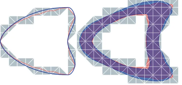
as approximations of the given hypersurface Γ and the neighborhood Dh _:= {x∈ U| |Φ(x)| < h} ; see Figure 1, for example. Note that Γ_h is a polygon whose facets are line segments ifn= 1 and a polyhedral surface whose facets consist of tri-angles or quadrilaterals ifn= 2. The corresponding decomposition of Γ_his in general not shape regular and can have arbitrary small elements.

Furthermore, we introduceF_h:U →Rn+1 _by

Fig. 1_{. A cartoon of the domains of the sharp interface (left) and the narrow band (right)}

method. The surfaceΓ, resp., the setDhis displayed in red, the approximationsΓ_h, resp.,D_hin blue, and the domainsU_hI, U_hB in gray.

whereF was defined in (2.3). From the properties ofF we infer that

p(F_h(x)) =p(x) and Φ(F_h(x)) =I_hΦ(x) ifF_h(x)∈U_δ,

(2.18)

F_h(x) =p(x) ifx∈Γ_h.

(2.19)

Lemma 2.1. There exists 0 < h₁ ≤ h₀ such that for 0 < h ≤h₁ the mapping F_h:D_h→Dh_{:={x∈U| |Φ(x)|< h}is bi-Lipschitz withF}

h(Γh) = Γ. Furthermore,

F_h−Id_L∞_(U)+hDFh−IL∞(U)≤ch2, (2.20)

|detDFh| −|∇IhΦ|

|∇Φ|

L∞(U)≤

ch2.

(2.21)

Proof. SinceF(p(x),Φ(x)) =xwe deduce with the help of (2.15)

|F_h(x)−x|=|F(p(x), I_hΦ(x))−F(p(x),Φ(x))| ≤c|I_hΦ(x)−Φ(x)| ≤ch2.

Differentiating the relationF_i(p(x),Φ(x)) =x_i,i= 1, . . . , n+ 1, we obtain

n+1

k=1

D_kF_i(p(x),Φ(x))p_k,xj(x) +∂Fi

∂s(p(x),Φ(x))Φxj(x) =δij, i, j= 1, . . . , n+ 1,

and hence

(2.22)

F_hi,xj(x) =

n+1

k=1

D_kF_i(p(x), I_hΦ(x))p_k,xj(x) +∂Fi

∂s (p(x), IhΦ(x))(IhΦ)xj(x)

=δ_ij+∂Fi

∂s(p(x),Φ(x))

I_hΦ−Φ

xj(x)

+

n+1

k=1

D_kF_i(p(x), I_hΦ(x))−D_kF_i(p(x),Φ(x))

p_k,xj(x)

+

∂F_i

∂s(p(x), IhΦ(x))− ∂F_i

∂s(p(x),Φ(x))

(I_hΦ)_xj(x)

=δ_ij+ Φxi(x)

|∇Φ(x)|2

I_hΦ−Φ

where |r_ij(x)| ≤ch2 in view of (2.15). This implies (2.20). In particular we deduce that F_h is bi-Lipschitz provided that h is sufficiently small, whereas the properties

F_h(D_h) =Dh_andF

h(Γh) = Γ follow from (2.18). Finally we deduce from (2.22) that

|detDF_h|= 1 + ∇Φ

|∇Φ|2 · ∇(IhΦ−Φ) +ch=

∇Φ· ∇I_hΦ

|∇Φ|2 +ch

= |∇IhΦ|

|∇Φ| − 1 2

∇IhΦ

|∇I_hΦ|−

∇Φ

|∇Φ|

2|∇IhΦ|

|∇Φ| +ch=

|∇I_hΦ|

|∇Φ| +dh,

where|ch|,|dh| ≤ch2proving (2.21).

We introduce μ_h : Γ_h → Rvia dσ(p(x)) = μ_h(x) dσ_h(x). It is well known (see Proposition 2.1 in [15], (3.37) in [34]) that

(2.23) |1−μh| ≤ch2 on Γ_h.

Using the properties of F_h together with the coarea formula and (2.9),(2.10), (2.11), (2.23) one can prove the following result on the equivalence of certain norms.

Lemma 2.2. There exist constantsc₁, c₂ >0 which are independent of h, such

that for all z∈H1(Γ)

c1ze_L2_(Γh)≤ z_L2_(Γ)≤c2ze_L2_(Γh),

c1√1

hz

e

L2(Dh)≤ zL2(Γ)≤c2

1

√

hz

e L2(Dh), c1∇ze_L2(Γh)≤ ∇ΓzL2(Γ)≤c2∇zeL2(Γh),

c1√1

h∇z

e

L2(Dh)≤ ∇ΓzL2(Γ)≤c2

1

√

h∇z

e L2(Dh).

If in addition z∈H2(Γ)then

c1√1

h

D2ze

L2(Dh)≤ zH2(Γ).

2.3. Variational form of elliptic equation and Strang’s second lemma. It is well known [1] that for everyf ∈L2(Γ) there exists a unique solutionu∈H2(Γ) of (1.1) which satisfies

(2.24) u_H2(Γ)≤cfL2(Γ).

Let us write (1.1) in weak form:

(2.25) a(u, ϕ) =l(ϕ) for allϕ∈H1(Γ),

where

a(w, ϕ) =

Γ

∇Γw· ∇Γϕ+wϕdσ, l(ϕ) =

Γ

f ϕdσ.

Next, suppose thatV_h is a finite–dimensional space andVe:={ve|v∈H1(Γ)}. Assume thata_h : (V_h+Ve)×(V_h+Ve)→ Ris a symmetric, positive semidefinite bilinear form which is, in addition, positive definite on V_h×V_h. Furthermore, let

l_h:V_h→Rbe linear. Then the approximate problem

has a unique solutionu_h∈V_h. Introducing

v_h:=a_h(v, v), v∈V_h+Ve,

we have by Strang’s second lemma

(2.27) ue−uh_h≤2 inf

vh∈Vh

ue−vh_h+ sup

φh∈Vh

|a_h(ue_{, φ}

h)−lh(φh)| φh_h .

3. Sharp interface method (SIF).

3.1. Setting up the method. Let us begin by observing that ifT ∈Thsatisfies

Hn_{(T ∩Γ}

h) > 0, then the following two cases can occur: (1) Γh∩int(T) = ∅, in

which caseHn(∂T∩Γ_h) = 0; (2)T∩Γ_h=∂T∩Γ_hin which caseT∩Γ_h is the face between two elements. We may now define a unique subset T_hI ⊂Th by taking all elements satisfying case 1 and in case 2 taking just one of the two elements T. The numerical method does not depend on which element is chosen. We may therefore conclude that there existsN ⊂Γ_hwithHn_{(N) = 0 and a subsetT}I

h ⊂Thsuch that

everyx∈Γ_h\N belongs to exactly oneT ∈TI

h. We then define

U_hI =

T∈TI h

T .

ClearlyUI

h ⊆Uδ ifhis small enough. We define the finite element spaceVhI by

V_hI ={φ_h∈C0(U_hI)|φ_h|T ∈P1(T) for each T ∈T_hI}. Note that∇φ_h is defined on Γ_h\N in view of the definition ofTI

h. In particular the

unit normalν_hto Γ_h is given by

(3.1) ν_h= ∇IhΦ

|∇I_hΦ| on Γh\N,

and we use (3.1) in order to extendν_h toUI

h. Let us next turn to the approximation

error for the spaceVI

h. Note that for a function z∈H

2_{(Γ) we havez}e_∈C0_{( ¯U} δ) so

thatI_hze _{is well–defined.}

Lemma 3.1. Let z∈H2(Γ). Then

(3.2) ze−I_hze_L2(Γh)+h∇(z

e_−I

hze)_L2(Γh)≤ch

2_z

H2(Γ). Proof. We first observe that Theorem 3.7 in [34] yields

(3.3) ze−I_hze_L2(Γh)+h∇Γh(ze−Ihze)_L2(Γh)≤ch

2_z

H2(Γ).

Hence, it remains to bound∇(ze_−I

hze)·νhL2(Γh). To do so, we start by considering

an elementT ∈TI

h. Then we see that

T∩Γh

|∇(ze−I_hze)·νh|2 dσ_h

≤2

T∩Γh

|∇ze·νh|2 dσ_h+ 2

T∩Γh

|∇(I_hze)·νh|2 dσ_h

≤2

T∩Γh

|∇ze·(ν_h−ν)|2 dσ_h+ch(T)−1

T

in view of (2.8) and the fact that Hn_{(T ∩Γ}

h)≤ch(T)−1Hn+1(T). Note that by

(3.1) and (2.15)

(3.4) ν−ν_hL∞(T)=

_|∇∇Φ_Φ|− ∇IhΦ |∇I_hΦ|

L∞(T)

≤ch(T)

so that

I1≤ch2

T∩Γh

|∇ze|2 dσ_h.

Furthermore, recalling (2.14) and using again (3.4)

I2≤ch(T)−1

T

|∇ze·(ν_h−ν)|2+|∇(ze−I_hze)|2dx≤chze2_H2(T).

We use the bounds forI1, I2and sum over all elementsT ∈T_hI, then apply Lemma 2.2 to see

Γ_h|∇

(ze−I_hze)·νh|2 dσ_h≤ch2∇ze2_L2_(Γh)+chze2_H2(Dc₁h)≤ch

2_z2

H2(Γ),

sinceT ⊂D_c1h for allT ∈ T_hI in view of (2.16).

3.2. The method. Let us write (1.3) in the form findu_h∈V_hI such that

(3.5) a_h(u_h, φ_h) =l_h(φ_h) for allφ_h∈V_hI,

where

a_h(w_h, φ_h) =

Γh

∇w_h· ∇φ_h+w_hφ_hdσ_h, l_h(φ_h) =

Γh

feφ_hdσ_h.

In order to verify that the symmetric bilinear form a_h is positive definite on

VI

h ×VhI we note thatah(φh, φh) = 0 implies that

Γh∩T

|∇φh|2+φ2_hdσ_h= 0 for allT ∈T_hI.

SinceHn_{(T ∩Γ}

h)>0 forT ∈ThI we infer that ∇φh = 0 and henceφh is constant

on these elements. Using again thatHn_(T∩Γ

h)>0 we deduce thatφh= 0 on each

T ∈TI

h so thatφh≡0 inVhI. Hence (3.5) has a unique solution uh∈VhI and

(3.6) uh_h=∇uh2_L2(Γh)+uh

2

L2(Γh)

1

2 _≤cfe

L2(Γh)≤cfL2(Γ). 3.3. Error analysis. The following error bounds hold.

Theorem 3.2. Let u be the solution of (1.1) and u_h the solution of the finite

element scheme (3.5). Then

Proof. In view of the definition of ·_h, (2.27), and Lemma 3.1 we have for

e_h:=ue_−u h

eh2_L2(Γ_h)+∇eh2L2(Γh)

1 2 (3.8)

≤2ue−I_hue2_L2(Γh)+∇(u

e_−I

hue)2_L2(Γh)

1 2

+ sup

φh∈VhI

|a_h(ue_{, φ}

h)−lh(φh)| φhh

≤chu_H2(Γ)+ sup

φh∈V_hI

|a_h(ue_{, φ}

h)−lh(φh)| φhh .

In order to estimate the second term we chooseφ_h∈VI

h, then forϕh:=φh◦Fh−1,

a_h(ue, φ_h)−l_h(φ_h) =a_h(ue, φ_h)−a(u, ϕ_h)+l(ϕ_h)−l_h(φ_h)≡I+II.

Using the transformation rule and (2.11) we obtain

Γ

∇Γu· ∇Γϕh+uϕh

dσ=

Γ_h

(∇Γu)◦p·(∇Γϕh)◦p+ (u◦p) (ϕh◦p)

μ_hdσ_h

=

Γh

(I+ ΦA)−1∇ue·(I+ ΦA)−1∇ϕe_h+ueϕe_hμ_hdσ_h.

(3.9)

Sinceϕe

h(x) =ϕh(p(x)) =φh(F_h−1(p(x))) we derive

∇ϕe_h(x) = [Dp(x)]T[DF_h−1(p(x))]T∇φ_h(F_h−1(p(x))) = [Dp(x)]T[DF_h(F_h−1(p(x)))]−T∇φ_h(F_h−1(p(x))).

We infer from (2.22) that

(3.10) (DF_h)−T =I− 1

|∇Φ|∇ηh⊗ν+Bh with |Bh| ≤ch 2_,

where η_h = I_hΦ−Φ. It follows from (2.19) that F_h−1(p(x)) = x, x ∈ Γ_h, which together with (2.9) implies

∇ϕe_h= (I−ν⊗ν)

I− 1

|∇Φ|∇ηh⊗ν

∇φ_h+q_h on Γ_h, |qh| ≤ch2|∇φh|.

Taking into account that∇ue_{·ν= 0 we therefore have}

∇ue· ∇ϕe_h=∇ue· ∇φ_h− 1

|∇Φ|(∇u

e_{· ∇η}

h)(∇φh·ν) +∇ue·qh on Γh.

Inserting this relation into (3.9) and recalling the definition ofa_hwe find that

|I| ≤

Γh

_∇ue· ∇φ_h−μ_h(I+ ΦA)−T(I+ ΦA)−1∇ue· ∇ϕe_h+|(μ_h−1)ueϕe_h|dσ_h

≤ch2ue_hφh_h+chueh

Γh

where we used (2.15), (2.23), and the fact thatϕe

h=φh on Γh. Similarly,

|II|=

Γf ϕhdσ−

Γ_hf

e_φ hdσh

≤

Γ_h|1−μh| |f

e_{| |φh|dσ} h

≤ch2fe_L2(Γ_h)φhh≤ch

2_f

L2(Γ)φhh.

Combining these estimates with (2.24) we have

(3.11) |a_h(ue, φ_h)−l_h(φ_h)| ≤ch2f_L2(Γ)φh_h+chfL2(Γ)

Γh

|∇φ_h·ν| dσ_h

for allφ_h∈V_hI, which inserted into (3.8) yields

(3.12) eh_L2_(Γh)+∇eh_L2_(Γh)≤chf_L2_(Γ).

In order to improve theL2-error bound we employ the usual Aubin–Nitsche argument. Denote byw∈H2(Γ) the solution of the dual problem

a(ϕ, w) =

Γ

e_hϕdσ for allϕ∈H1(Γ) withe_h=e_h◦F_h−1,

which satisfies

(3.13) w_H2(Γ)≤cehL2(Γ).

We have in view of (1.3)

(3.14)

eh2_L2(Γ)=a(eh, w) =

a(e_h, w)−a_h(e_h, we)

+a_h(e_h, we−I_hwe) +a_h(ue, I_hwe)−l_h(I_hwe)

≡I+II+III.

Similarly as above we deduce with the help of (3.12) and Lemma 2.2

|I| ≤cheh_hwe_h≤ch2f_L2(Γ)wH1(Γ).

Next, Lemma 3.1 and (3.12) imply

|II| ≤ eh_hwe−I_hwe_h≤ch2f_L2_(Γ)w_H2_(Γ).

Finally, (3.11), the fact that∇we_{·ν= 0, and Lemma 3.1 yield}

|III| ≤ch2f_L2(Γ)Ihweh+chfL2(Γ)

Γh

|∇(I_hwe−we)·ν|dσ_h

≤ch2f_L2(Γ)wH2(Γ).

Inserting the above estimates into (3.14) and recalling (3.13) we obtain

eh_L2(Γ)≤ch2fL2(Γ),

which together with Lemma 2.2 completes the proof sinceee

4. Narrow band method (NBM).

4.1. Setting up the method. Recalling the definition ofD_h(2.17), we consider

TB

h ={T ∈Th|Hn

+1_(T∩D

h)>0} and UhB=

T∈TB h

T .

We define the finite element spaceVB

h on the triangulationThB by

V_hB={φ_h∈C0(U_hB)|φ_h|T ∈P1(T) for eachT ∈T_hB}.

Let us first examine the approximation error for the spaceVB h .

Lemma 4.1. We have for each function z∈H2(Γ)that I_hze∈VB

h satisfies

(4.1) √1

hz

e_−I

hzeL2(Dh)+

√

h∇(ze−I_hze)_L2(Dh)≤ch

2_z

H2(Γ).

Proof. We infer from (2.14) and Lemma 2.2 that

1

hz

e_−I

hze2L2(Dh)+h∇(z

e_−I

hze)2L2(Dh)

≤

T∩Dh=∅

1

hz

e_−I

hze2L2(T)+h∇(ze−Ihze)2L2(T)

≤ch3

T∩Dh=∅

ze2_H2(T)≤ch

3_ze2

H2(D(1+c1)h)≤ch

4_z2

H2(Γ),

sinceT ⊂D_(1+c1)h for allT∩D_h=∅ in view of (2.16).

4.2. The method. Let us write (1.5) in the form findu_h∈V_hB such that

(4.2) a_h(u_h, φ_h) =l_h(φ_h) for allφ_h∈V_hB,

where

a_h(w_h, φ_h) = 1 2h

Dh

∇w_h· ∇φ_h+w_hφ_h|∇I_hΦ|dx,

l_h(φ_h) = 1 2h

Dh

feφ_h|∇I_hΦ|dx.

Note that the factors 1_h in each of the above terms are there to aid the notation for the error analysis. In a similar way as for SIF one can verify thata_h is positive definite onV_hB ×V_hB. Hence, the finite element scheme (4.2) has a unique solution

u_h∈VB

h which satisfies

(4.3) uh_h=

1 2h

Dh

|∇uh|2+u2_h|∇I_hΦ|dx

1 2

≤cf_L2_(Γ).

4.3. Error analysis. Before we prove our main error bound we formulate a technical lemma which will be helpful in the error analysis.

Lemma 4.2. Suppose that u∈H2(Γ)is a solution of(1.1). Then,

a_h(ue, φ) = 1 2h

Dh

feφ◦F_h−1|∇Φ|dx+ 1 2h

Dh

(∇ue·∇η_h)(∇φ·ν)|∇IhΦ|

for allφ∈H1(D_h), where η_h=I_hΦ−Φand

|S, φ| ≤Ch2u_H2(Γ)φh.

Proof. To begin, we derive from (2.12) and (1.1) that

(4.4) − 1

|∇Φ|∇ ·

|∇Φ| ∇ue+ue=fe+R in U_δ,

where

(4.5) R(x) =−Φ(x)

⎛ ⎝n+1

k,l=1

b_lk(x)D_lD_ku(p(x)) +

n+1

k=1

c_k(x)D_ku(p(x))

⎞ ⎠.

We multiply (4.4) by φ◦F_h−1|∇Φ|, φ ∈ H1(D_h), and integrate over Dh_{. Since} ∂ue

∂ν = 0 on∂Dh we obtain after integration by parts

(4.6)

Dh

∇ue· ∇(φ◦F_h−1)|∇Φ|dx+

Dh

ueφ◦F_h−1|∇Φ| dx

=

Dh

feφ◦F_h−1|∇Φ|dx+

Dh

R φ◦F_h−1|∇Φ|dx.

Observing that∇(φ◦F_h−1) = [(DF_h)−T◦F_h−1]∇φ◦F_h−1, the transformation rule and Lemma 2.1 imply that

I:=

Dh

∇ue·∇(φ◦F_h−1)|∇Φ|dx=

Dh

∇ue◦Fh·(DF_h)−T∇φ|∇Φ◦Fh| |detDFh|dx.

Recalling (2.7) and (2.18) we have

(4.7) ze(x) =z(p(x)) =z(p(F_h(x)) =ze(F_h(x)),

from which we deduce by differentiation

(4.8) ∇ze◦F_h= (DF_h)−T∇ze,

so that

I=

Dh

(DF_h)−T∇ue·(DF_h)−T∇φ|∇Φ◦Fh| |detDFh|dx.

Recalling (3.10), we find with the help of∇ue·ν= 0 that

(DF_h)−T∇ue=∇ue+Bh∇ue, (DF_h)−T∇φ=∇φ− 1

|∇Φ|(∇φ·ν)∇ηh+Bh∇φ,

where|Bh| ≤ch2. Furthermore, Lemma 2.1 implies that

|∇Φ◦Fh| |detDFh|=|∇I_hΦ|+γ_h, where |γh| ≤ch2,

so that in conclusion

I=

Dh

∇ue· ∇φ|∇I_hΦ| dx−

Dh

(∇ue· ∇η_h)(∇φ·ν)|∇IhΦ|

|∇Φ| dx+R 1

where

R1_h, φ≤ch2∇ue_L2(Dh)∇φL2(Dh)≤ch

3_u

H2(Γ)φh,

in view of Lemma 2.2 and the definition of·_h. Similarly, (4.7) and (2.21) yield

Dh

ueφ◦F_h−1|∇Φ|dx=

Dh

ueφ|∇I_hΦ|dx+R_h2, φ

with R2_h, φ ≤ ch3u_H2(Γ)φh. Inserting the above identities into (4.6) and

dividing by 2hwe derive (4.9)

a_h(ue, φ) = 1 2h

Dh

feφ◦F_h−1|∇Φ|dx+ 1 2h

Dh

R φ◦F_h−1|∇Φ|dx

+ 1 2h

Dh

(∇ue· ∇η_h)(∇φ·ν)|∇IhΦ|

|∇Φ| dx− 1 2hR

1

h, φ −

1 2hR

2

h, φ.

In order to rewrite the integral overDh_{we note thatF(·, s) maps Γ onto Γ}

s={Φ =s}

and that dσ_s = (1 +O(s)) dσ_p, where dσ_s, dσ_p are the surface elements of Γ_s,Γ respectively. The coarea formula then yields for integrableg:Dh→R

Dh

g(x) dx=

_h

−h

Γs

g(x) 1

|∇Φ(x)|dσsds=

_h

−h

Γ

g(F(p, s))μ(p, s) dσ_pds

where μ(p, s)− 1

|∇Φ(F(p, s))|

≤C|s|, |s|< h, p∈Γ.

(4.10)

Hence,

Dh

R φ◦F_h−1|∇Φ|dx

=

_h

−h

Γ

R◦F φ◦F_h−1◦F |∇Φ◦F|μdσ_pds

=

_h

−h

Γ

R◦F φ◦F_h−1◦Fdσ_pds+

_h

−h

Γ

r φ◦F_h−1◦Fdσ_pds

≡T1+T2,

wherer(p, s) =R(F(p, s))μ(p, s)|∇Φ(F(p, s))| −1. In order to treatT1 we deduce from (4.5) and the fact that Φ(F(p, s)) =sthat

R(F(p, s)) =−s

⎛ ⎝n+1

k,l=1

b_lk(F(p, s))D_lD_ku(p) +

n+1

k=1

c_k(F(p, s))D_ku(p)

⎞ ⎠.

Since₋h_hsds= 0, the first term inT1can be written as

− _h −h Γ n+1 k,l=1

sD_lD_ku(p)

b_lk(F(p, s))φ◦F_h−1(F(p, s))−b_lk(p)φ◦F_h−1(p)

dσ_pds.

Treating the second term in T1 in the same way and observing that p=F(p,0) we deduce with the help of the fundamental theorem of calculus that

|T1| ≤ch52_u

H2(Γ)

Dh

∇φ◦F_h−12+φ◦F_h−12

dx

1 2

Next, we infer from (4.5) and (4.10) that

|r(p, s)| ≤cs2|∇Γu(p)|+D2Γu(p),

so that

|T2| ≤Ch52u_H2(Γ)

Dh

φ◦F_h−12 dx

1 2

≤Ch3u_H2(Γ)φh.

The result now follows from (4.9) together with the bounds onR1_h andR2_h.

Theorem 4.3. Let u be the solution of (1.1) and u_h the solution of the finite

element scheme (4.2). Then

(4.11) ue−uh_L2(Γ_h)+h

1 2h

Dh

|∇(ue−u_h)|2|∇I_hΦ|dx

1 2

≤ch2f_L2(Γ).

Proof. Let us writee_h:=ue_−u

h. We infer from (2.27) and Lemma 4.1 that

(4.12) eh_h≤chu_H2(Γ)+ sup

φh∈V_hB

|a_h(ue_{, φ}

h)−lh(φh)| φh_h .

The second term on the right-hand side can be estimated with the help of Lemma 4.2. The transformation rule together with (4.7) yields

1 2h

Dh

feφ_h◦F_h−1|∇Φ| dx= 1 2h

Dh

fe◦F_hφ_h |∇Φ◦Fh| |detDFh|dx,

so that we deduce from Lemma 4.2

a_h(ue, φ_h)−l_h(φ_h) = 1 2h

Dh

(∇ue· ∇η_h) (∇φ_h·ν)|∇IhΦ|

|∇Φ|

+ 1 2h

Dh feφ_h

|∇Φ◦Fh| |detDFh| − |∇I_hΦ|

dx+S, φh.

Using (2.21), (2.15), (2.24), and Lemmas 2.1 and 2.2 we infer that for φ_h∈V_hB

|a_h(ue, φ_h)−l_h(φ_h)| ≤c∇ue_L2(Dh)

Dh

|∇φ_h·ν|2dx

1 2

+chfe_L2(Dh)φhL2(Dh)+ch

2_u

H2(Γ)φhh

(4.13)

≤chf_L2(Γ)

1 2h

Dh

|∇φ_h·ν|2dx

1 2

+ch2f_L2(Γ)φhh,

so that (4.12) implies the following intermediate result:

(4.14) eh_h=

1 2h

Dh

|∇eh|2+e2_h|∇I_hΦ|dx

1 2

≤chf_L2_(Γ).

In order to improve theL2-error bound we definee_h:=e_h◦F_h−1 as well as

E_h(p) := 1 2h

h

−h

withF as above. We denote byw∈H2(Γ) the unique solution of

−ΔΓw+w=E_h on Γ,

which satisfies

(4.15) w_H2(Γ)≤cEh

L2(Γ)

.

Similarly to (4.4) the extensionwe solves

− 1 |∇Φ|∇ ·

|∇Φ| ∇we+we=E_he+R in U_δ,

where R is obtained from (4.5) by replacingu byw. Using the transformation rule together with (4.10) we obtain

_E h

2

L2(Γ)= 1 2h h −h Γ

Ehe_h◦Fdσ_pds= 1 2h h −h Γ

E_he◦Fe_h◦F|∇Φ◦F|μdσ_pds

+ 1 2h _h −h Γ

E_he_h◦F(1− |∇Φ◦F|μ) dσ_pds

= 1

2h

Dh

E_hee_h◦F_h−1|∇Φ|dx

+ 1 2h _h −h Γ

E_he_h◦F(1− |∇Φ◦F|μ) dσ_pds.

The first term can be rewritten with the help of Lemma 4.2 (applied towinstead of

u) to give

_E h

2

L2(Γ)=ah(w

e_{, e}

h)− S, e h −

1 2h

Dh

(∇we· ∇η_h)(∇e_h·ν)|∇IhΦ|

|∇Φ| dx

+ 1 2h h −h Γ

E_he_h◦F(1− |∇Φ◦F|μ) dσ_pds≡

4

k=1

I_k.

In view of Lemma 4.1, (4.13), the fact that∇we_{·ν = 0, and (4.14) we have}

|I1|+|I2| ≤ |ah(we−Ihwe, eh)|+|ah(ue, Ihwe)−lh(Ihwe)|+|S, e h| ≤chw_H2_(Γ)eh_h+ch2f_L2_(Γ)Ihweh

+chf_L2(Γ)

1 2h

Dh

|∇(I_hwe−we)·ν|2dx

1 2

+ch2w_H2(Γ)ehh ≤ch2f_L2(Γ)wH2(Γ).

Furthermore, (2.15), (4.10), and (4.14) imply

|I3|+|I4| ≤ch

we_h+E_h

L2(Γ)

eh_h≤ch2f_L2(Γ)

w_H2(Γ)+Eh L2(Γ)

,

so that we obtain together with (4.15)

_E h

L2(Γ)≤ch

2_f

Next, sinceF(p,0) =pwe may write forp∈Γ

E_h(p)−e_h(p) = 1 2h

h

−h

s

0 ∇

e_h(F(p, τ))· ∂F

∂s(p, τ) dτds,

and hence we obtain with the help of (4.14)

_E h−eh

L2(Γ)≤c

√

h

Dh

|∇eh|2dx

1 2

≤ch∇eh_h≤ch2f_L2_(Γ).

In conclusion we deduce that

eh_L2(Γh)≤cehL2(Γ)≤ _E

h−eh L2(Γ)

+E_h

L2(Γ)≤

ch2f_L2(Γ)

and the theorem is proved.

5. A hybrid method for equations on evolving surfaces.

5.1. The setting. The aim of this section is to combine ideas employed in sections 3 and 4 for the stationary problem in order to develop a finite element method for an advection–diffusion equation on an evolving hypersurface in which there is an underlying conservation law with a diffusive flux, [18]. More precisely, let (Γ(t))_t∈[0,T] be a family of compact, connected smooth hypersurfaces embedded inRn+1 _forn=

1,2. We suppose that

Γ(t) ={x∈ N(t)|Φ(x, t) = 0}, where∇Φ(x, t)= 0, x∈ N(t),

and N(t) is an open neighborhood of Γ(t). We assume that N(t) is chosen so small that we can construct the function p(·, t) as in section 2.1. Given a velocity field

v(·, t) : Γ(t)→ Rn+1_{, not necessarily in the normal direction, we then consider the}

following initial value problem

∂•u+u∇Γ·v−ΔΓu=f on

t∈(0,T)

Γ(t)× {t},

(5.1a)

u(·,0) =u0 on Γ(0). (5.1b)

Here, ∂•η denotes the material derivative of a function η : _t∈(0,T)Γ(t)× {t} → R

which is given by

∂•η =∂_tη+v· ∇η

ifη is extended into a neighborhood of_t∈(0,T)Γ(t)× {t}.

5.2. The method. In order to discretize the above problem we choose a parti-tion 0 =t0 < t1 <· · · < t_N =T of [0, T] withτ_m :=t_m+1−t_m, m= 0, . . . , N−1, and τ := max_m=0,...,N−1τm. Also, let Th be an unfitted regular triangulation with

mesh sizehof a region containingN(t), t∈[0, T]. Form= 0,1, . . . , N we set

Γm_h ={x∈ N(t_m)|I_hΦ(x, t_m) = 0} and D_hm={x∈ N(t_m)| |I_hΦ(x, t_m)|< h},

as well as

Tm

h :={T ∈Th|Hn

+1_(T∩Dm

h)>0} and Uhm:=

Here we assume that 0 < h ≤ h0, where h0 is chosen so small that there exists

c0, c1>0 such that

c0≤ |∇IhΦ(x, t)| ≤c1, (x, t)∈

t∈(0,T)

N(t)× {t}.

Finally, we introduce

V_hm={φ_h∈C0(U_hm)|φh|T ∈P1(T) for each T∈T_hm}.

In what follows we shall frequently use the abbreviationzm_{(x) :=z(x, t} m).

In order to motivate our method we fix m∈ {0,1, . . . , N−1} and let Ψ be the solution of

Ψ_t(x, t) +DΨ(x, t)ve(x, t) = 0, Ψ(x, t_m+1) =x,

where ve_{(x, t) := v(p(x, t), t). For a sufficiently smooth function ϕ: N(t}

m+1) → R

we define η(x, t) :=ϕ(Ψ(x, t)). Clearly,η(·, t_m+1) =ϕand a short calculation shows that∂•η= 0. Assuming that uis a solution of (5.1a) we obtain with the help of the Leibniz formula and integration by parts

d dt

Γ(t)

uηdσ_|t=tm+1 =

Γ(tm+1)

∂•(uη) +uη∇Γ·vdσ

=

Γ(tm+1)

ϕ∂•u+u∇Γ·vdσ

=

Γ(tm+1)

ϕΔΓu+ϕfdσ

=−

Γ(tm+1)

∇Γu· ∇Γϕdσ+

Γ(tm+1)

f ϕdσ.

Since Ψ(·, t_m+1)≡id, a Taylor expansion shows that

Ψ(x, t_m) = Ψ(x, t_m+1−τ_m)≈x−τ_mΨ_t(x, t_m+1)

=x+τ_mDΨ(x, t_m+1)ve,m+1(x) =x+τmve,m+1(x).

Thus we may approximate the left-hand side of the above relation by

d dt

Γ(t)

uηdσ_|t=tm+1≈ 1

τ_m

Γ(tm+1)

um+1ϕdσ−

Γ(tm)

umϕ(·+τ_mve,m+1) dσ

.

The above calculations motivate the following scheme, in which we use the narrow band approach in order to discretize the elliptic part. Givenum

h ∈Vhm, m= 1, . . . , N−

1, findum_h+1∈V_hm+1 such that

(5.2)

Γm+1

h

um_h+1φ_hdσ_h−

Γm h

um_hφ_h(·+τ_mve,m+1) dσ_h

+τm 2h

Dm_h+1

∇um_h+1· ∇φ_h|∇I_hΦm+1|dx=τ_m

Γm+1

h

fe,m+1φ_hdσ_h

5.3. Mass conservation. An important property of solutions of (5.1a) is con-servation of mass in the case that _Γ(t)f(·, t) dσ = 0. The following lemma shows that our numerical scheme preserves this property under some mild constraints on the discretization parameters. In fact this discrete conservation law is a remarkable property of the scheme and relies on the use of both a sharp interface and a narrow band approach.

Lemma 5.1. _{Let u}m

h ∈Vhm, m = 1, . . . , N, be the solutions of (5.2)in the case

Γm+1

h f

e,m+1_dσ

h= 0, m= 0, . . . , N−1. Then provided that0< h≤h1andτ≤γ√h

(5.3)

Γm h

um_h dσ_h=

Γ0

h

u0_hdσ_h.

Proof. Let us first observe that

(5.4) {x+τ_mve,m+1(x)|x∈Γm_h} ⊂U_hm+1, m= 0, . . . , N−1,

provided thath, τare sufficiently small. To see this, letx∈Γm

h and choose an element

T ∈Th such thatx∈T. Then,

Φm+1(x+τ_mve,m+1(x)) = Φm(x) +τm∇Φm(x)·ve,m+1(x) +τ_mΦ_t(x, t_m) +R_m(x),

where|R_m(x)| ≤cτ_m2. Observing that Φ_t+∇Φ·v= 0 on_t∈(0,T)Γ(t)× {t}we write

∇Φm(x)·ve,m+1(x) + Φ_t(x, t_m)

=∇Φm(x)·vm+1(pm+1(x)) + Φ_t(x, t_m)

=∇Φm(x)− ∇Φm+1(pm+1(x))·vm+1(pm+1(x))

+ Φ_t(x, t_m)−Φ_t(pm+1(x), t_m+1),

so that

Φm+1(x+τ_mve,m+1(x))≤ |Φm(x)|+cτ_mx−pm+1(x)+cτ_m2

≤ |Φm(x)|+cτ_mΦm+1(x)+cτ_m2 ≤c(h2+τ_m2),

in view of (2.5) and since|Φm(x)|=|Φm(x)−I_hΦm(x)| ≤ch2. As a result,

(I_hΦm+1)(x+τ_mve,m+1(x))≤I_hΦm+1−Φm+1

L∞+c(h

2_+τ2

m)≤c(h2+τm2)< h

provided that 0< h ≤h1 andτ ≤γ

√

h. Hence,x+τ_mve,m+1_(x)∈Dm+1

h ⊂Um

+1

h

proving (5.4). The result of the lemma follows from inserting φ_h ≡1 ∈ V_hm+1 into (5.2) and using (5.4) together with our assumption that_Γm+1

h f

e,m+1_dσ

h= 0.

6. Numerical experiments.