Operator Product Formula for a Special Macdonald Function

(1)

http://www.scirp.org/journal/am

ISSN Online: 2152-7393 ISSN Print: 2152-7385

DOI: 10.4236/am.2018.94033 Apr. 30, 2018 459 Applied Mathematics

Operator Product Formula for a Special

Macdonald Function

Lifang Wang

2

, Ke Wu

1

, Jie Yang

1

1_{School of Mathematical Sciences, Capital Normal University, Beijing, China} 2_{School of Mathematics and Statistics, Henan University, Kaifeng, China}

Abstract

In this paper, we construct two sets of vertex operators S+ and S− from a

direct sum of two sets of Heisenberg algebras. Then by calculating the vacuum expectation value of some products of vertex operators, we get Macdonald function in special variables i1

i

x =t− (i=0,1, 2,). Hence we obtain the op-erator product formula for a special Macdonald function

(

1

)

1, , , n ; , Pλ t t − q t when n is finite as well as when n goes to infinity.

Keywords

Macdonald Function, Vertex Operator, Heisenberg Algebra

1. Introduction

The study of topological string on Calabi-Yau manifolds is interested in mathematical physics for many years. It was found that gauge theories with certain gauge groups can be geometrically engineered from some Calabi-Yau threefolds, and the topological string partition functions on such spaces are related to instanton sums in gauge theories [1].

The topological vertex formalism provides a powerful method to calculate the topological string partition function for non-compact toric Calabi-Yau 3-fold. By transfer matrix approach, A. Okounkov, N. Reshetikhin and C. Vafa proposed the topological vertex Cλµν using Schur and skew Schur functions

[2]:

( )

( )2

( )

(

)

( )

/ /

t

t t

C q q s q s q s q

κ µ

ρ ν ρ ν ρ

λµν _ν _{λ η} µ η

η

− − − − −

=

∑

where λ µ ν, , are Young diagrams, λt denotes the transpose of λ, and How to cite this paper: Wang, L.F., Wu,

K. and Yang, J. (2018) Operator Product Formula for a Special Macdonald Function. Applied Mathematics, 9, 459-471.

https://doi.org/10.4236/am.2018.94033

Received: April 4, 2018 Accepted: April 27, 2018 Published: April 30, 2018

http://creativecommons.org/licenses/by/4.0/

(2)

DOI: 10.4236/am.2018.94033 460 Applied Mathematics

(

1 2 , 3 2 , 5 2 ,

)

ρ= − − − _ _{. The topological vertex} C_λµν has a nice interpretation by statistical mechanics of the melting crystal model [2] [3]. In this paper two sets of vertex operators constructed specifically by the annihilation and creation generators of Heisenberg algebra play important roles in realizing Schur and skew Schur functions.

On the other hand, gauge theory partition function is a function with two equivariant parameters. In 2007, based on the arguments of geometric engineering, concerning the K-theoretic lift of the Nekrasov partition functions, A. Iqbal, C. Kozçaz and C. Vafa introduced a refined version of topological vertex [4]. In this refinement, one more parameter t comes in and the theory seems to be deeply related to a Macdonald function with special variables, or what we call a special Macdonald function, P tλ

(

−ρ; ,q t

)

:

( )

(

)

(

)

(

)

2 2

2

/ /

, t ; ,

t t

q

C t q t P t q t

t q

s t q s t q

t

µ ν

κ µ ρ

λµν _ν

η λ µ

ρ ν ν ρ

µ η λ η

η +

−

+ −

− − − −

  =  _{ }

  × _{ }  

∑

where 2 2

i i

λ =

∑

λ . Moreover H. Awata and H. Kanno proposed another formula [5] which is expressed entirely in terms of the special (skew) Macdonald functions:

( )

(

)

( )

(

)

(

)(

)

1

1 2 1 2 /

/

, ; , ,

; , ; , ,

t t t C q t P t q t f q t

P t q t q P q t q t q t

ν ρ

µλ λ ν

σ ν

λ ρ λ ρ

ν σ µ σ

σ

ι

−

=

×

∑

−

where

( ) ( )

( )

2 ( ) 2

, 1

t

n n

f_λ q t = − λ q λ +λ t− λ λ− and ι is the involution on the algebra of symmetric functions defined by ι

( )

pn = −pn, here

( )

1

n n i i p x =

∑

∞₌x . Although C_λµν

( )

t q, and Cνµλ

( )

q t, have different expressions, they are supposed to give the same result.

Therefore it seems that the key problem is to change Schur function for the unrefined case to Macdonald function for the refined one. Hence to find a vertex operator formalism for the refined topological vertex will be interesting. The essential step is to realize the special Macdonald function P t_λ

(

−ρ; ,q t

)

. However a vertex operator formalism for P tλ

(

−ρ; ,q t

)

does not exist so far.

In this paper, we get the operator product formula for the special Macdonald

function

(

1

)

1, , , n ; ,

Pλ t t − q t . We also extend this formula to the case when n goes to infinity.

2. Preliminaries

2.1. Notations

• : the set of rational numbers;

• 

( )

q t, : the field of rational functions of q, t over ;

• The q infinite product:

( )

(

)

0

; : 1 n

n

x q _∞ xq

≥

(3)

2.2. Partitions

A partition is any (finite or infinite) sequence λ=

(

λ λ1, 2,,λr,

)

of

non-negative in decreasing order: λ λ1≥ 2≥≥λr≥ and containing only finitely many non-zero terms. We denote by λ _{the size of the partition, i.e.}

i i

λ =

∑

λ _{and by}l

( )

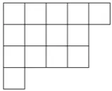
λ the number of non-zero λ_i. The set of all partitions is denoted by .

A pictorial representation of a partition λ is called 2D Young diagram , it can be obtained by placing λi boxes at the i-th row. For example, Figure 1 represents a partition λ=

(

5, 4, 4,1

)

.

The transpose of λ is denoted by λt_,

(

)

1, 2,

t t t

λ = λ λ  , here

{

}

Card | t

j i i j

λ

=

λ

≥ . For example, the transpose of λ=

(

5, 4, 4,1

)

is

(

4, 3, 3, 3,1

)

t

λ

= _.

We denote by

( )

2

,

s= i j ∈ for each square of a partitionλ, here 1≤ ≤j λi. For each square s=

( )

i j, ∈λ, let

( )

,

( )

t ,

( )

( ) ( )

1,

i j

a s = −

λ

j l s =

λ

−i h s =a s +l s +

( )

1,

( )

1.

a s′ = −j l s′ = −i

The numbers a s

( )

and a s′

( )

may be called respectively the arm-length and the arm-colength of s, and l s

( )

, l s′

( )

the leg-length and the leg-colength.

2.3. Macdonald Function

We define a scalar product

( )

,

1

, ,

1 i

i

l

q t

i

q

p p z

t

λ λ

λ µ δλµ λ λ

= − =

−

∏

(1)

here

=

!

1

i i m

i

m

i

z

∏

≥

λ , where mi =mi

( )

λ is the number of parts of λ equal to i;

1 2

p_λ =p p_λ _λ  for each partition λ=

(

λ λ₁, ₂,

)

and _r _ir i p =

∑

x .

Macdonald function P x q t_λ

(

; ,

)

depends rationally on two parameters q t, , i.e. P x q tλ

(

; ,

)

∈ Λ ⊗

( )

q t, , here

[

1, , ,

]

n S n

x x

Λ =   and ⊗_ means

tensor product over



. They are characterized by the following two properties[6]:

1) P x q t_λ

(

; ,

)

is of the form: P_λ =m_λ+

∑

_{µ λ}_< u m_λµ _µ, where u_λµ∈

( )

q t, ;

2) , _, 0

q t

P P_λ _µ = , if λ µ≠ .

When q=t, P x q tλ

(

; ,

)

reduce to the schur function sλ.

[image:3.595.333.413.636.701.2]

In particular,

(4)

(

)

( ) ( ) ( )

( ) ( )

1

1, , , ; , ,

1

a s n l s n

n

a s l s s

q t

P t t q t t

q t

λ λ

λ

′ −′ −

+ ∈

− =

−

∏

 (2)

here l

( )

λ ≤n and

( )

(

)

1

= 1 _i

i

n λ

∑

_≥ i− λ . Let n→ ∞,

(

)

( )

( ) ( )1

1

1, , , , ; , .

1

n n

a s l s s

P t t q t t

q t

λ λ

λ +

∈ =

−

∏

  (3)

3. Operator Product Formula for

(

n

)

P

_λ

1, ,

t



,

t

−1

; ,

q t

.

3.1. Algebra

B

a b,

We introduce an algebra Ba b, generated by bosons

{ }

an n∈\ 0{ } and

{ }

bn n∈\ 0{ },

they satisfy the following relations:

[

am,an

]

=mδm n+,0

[

b bm, n

]

=mδm n+,0and

[

a bm, n

]

=0, for∀m n, ∈\ 0 .

{ }

Let 0 be the vacuum state which satisfies the conditions a_n 0 =0

(

n>0

)

and b_n 0 =0

(

n>0

)

. For a partition λ=

(

λ λ₁, ₂,

)

, we use a short notation

1 2

0 0

a_λ =a a_{λ λ}  .

The bosonic Fock space  is generated from the vacuum state:

{

}

: span= a b−_λ −_µ 0 : ,λ µ∈ .

 

The dual vacuum state 0 is defined by the conditions 0an=0 0

(

n<

)

and 0 b_n =0 0

(

n<

)

. The dual boson Fock space * is generated by the dual vacuum state:

{

}

*

: span 0= a b_{λ µ}: ,λ µ∈ .

 

There is a paring *_× _→



  denoted by

(

u ,v

)

 u v between two spaces, defined by the following properties:

(

)

(

)

, 0 0 =1, u a v = u a v for alla∈Ba b.

3.2. The Vertex Operators

To construct the vertex realization for

(

1

)

1, , , n ; ,

P_λ t t − q t , we propose two sets of vertex operators depending on q and t.

We define

( )

(

)

12

1 1

exp 1 i ,

n n i

i n

n

A t q t a

n

λ

λ ∞ −

+

=

 _ _ 

 

=  − _ _ 

 

 



∑

 (4)

( )

12

1

1 1

exp .

1

i n i

i n n

n

A q t a

n q

λ

λ ∞ − −

− −

=

 _ _ 

 

= − _ _ 

− _ _

 



∑

 (5)

Since

(

)

1 1

2 2

1 1

1 1 1

1 ,

1

i j

n m

n i j

n m m

n m

t q t a q t a

n m q

λ λ

∞ ₋ ∞ ₋

− −

= =

 _ _ _ _ 

 − _ _ − _ _ 

−

 _ _ _ _ 

(5)

[

]

1 1

2 2

1 1

1 0

1 1 1

, 1

1

ln ,

1

i j

j i

n m

n

i j

n m m

n m

m i j m i j m

t

q t q t a a

n m q

q t

λ λ

∞ ∞ ₋ ₋

−

= =

− + −

∞

− + − +

=

   

−

= − _  _{ } _

− _ _{ } _

 ₋ 

 

=  

−

 

 

∑∑

∏

we can obtain

( )

(

)

(

)

( )

1 0

1 1 1

;

. ;

j i

m i j

i j _{m i j} j i m

i j

j i i j

q t

A A A A

q t

q t q

A A

q t q

λ λ

λ λ λ λ

λ λ

− + −

∞

+ − − + − + − +

=

− −

∞

− +

− − +

∞

− =

−

=

∏

(6)

We define another set of vertex operators

( )

(

)

1

exp 1 n n ,

n n

B x t x b

n

∞ +

=

 

=  − 



∑

 (7)

( )

1

1 1

exp .

1

n n n n

B x x b

n q

∞

− −

=

 

=  ₋ 



∑

 (8)

Since

(

)

[

]

1 1

0

1 1 1

1 ,

1 1 1 1

, 1

1

ln ,

1

n n m

n m m

n m

n n m

n m m

n m

m m m

t x b y b

n m q

t

x y b b n m q

q txy q xy

∞ ∞

−

= =

∞ ∞

−

= =

∞

=

 

−

 ₋ 

 

− =

−

 − 

=  ₋ 

 

∑

∑∑

∏

likewise we obtain

( ) ( )

(

)

(

)

( ) ( )

0 1 1

;

. ;

m m m

q txy

B x B y B y B x

q xy txy q

B y B x xy q

∞

+ − − +

=

∞

− +

∞

− =

−

=

∏

(9)

3.3. Operator Product Formula for

(

n

)

P

_λ

1, ,

t



,

t

−1

; ,

q t

With the help of the vertex operator A₊

( )

λ_i ,A₋

( )

λ_i ,B₊

( )

x ,B₋

( )

x , we define vertex operators S₊

( )

i and S₋

( )

i as follows:

( )

(

)

12 12

1 1

exp 1 i ,

n n

n i i

n n

n

S i t q t a q t b

n

λ

∞ ₋

+

=

 _ _ _ _ 

  

=  − _ _ +_ _ 

   

 _ _



∑



(10)

and

( )

12 12

1

1 1

exp .

1

i

n n

i i

n n

S i q t a q t b

n q

λ

∞ ₋ ₋

− −

− − −

=

 _ _ _ _ 

  

= − ₋ _ _ −_ _ 

   

 _ _



∑



(11)

(6)

( ) ( ) (

1

) (

1

)

( ) ( ) ( ) ( )

2 2 1 1 .

S₋ n S₊ n S₋ n− S₊ n− S₋ S₊ S₋ S₊ (12) After some careful computation via the commutative relation (6) and (9), the Formula (12) is equal to

(

)

(

)

(

)

(

)

( ) (

)

( ) ( ) ( ) (

)

( ) ( )

1

1 1

; ;

1 2 1 1 2 1

j i

i j i j i j i j j i n

q t q t q

S n S n S S S n S n S S

λ λ

− − − +

∞ ∞

− − + −

≤ < ≤

∞ ∞

− − − − + + + +

× − −

∏

 

Using the identity (we will prove it in the appendix)

(

)

(

)

(

)

(

)

( ) ( ) ( ) ( )

1

1 1

1

; ; ₁

1

; ;

j i

i j i j

a s n l s

a s l s

i j i j

j i n s

q t q t q _q _t

q t

q t q t q

λ λ

λ

− − − + _′ ₋_′

∞ ∞

+

− − + −

≤ < ≤ ∈

∞ ∞

− =

−

∏

(13)

we get the vacuum expectation value of this operator product formula

( ) ( ) (

) (

)

( ) ( ) ( ) ( )

( ) ( ) ( ) ( )1

0 1 1 2 2 1 1 0

1

. 1

a s n l s a s l s s

S n S n S n S n S S S S

q t q t

λ

− + − + − + − +

′ −′

+ ∈

− −

− =

−

∏



(14)

In other words,

( ) ( ) (

) (

)

( ) ( ) ( ) ( )

( )

(

1

)

0 1 1 2 2 1 1 0

1, , , ; , .

n n

t λ P_λ t t q t

− + − + − + − +

− −

=



 (15)

Therefore we get the operator product formula for

(

1

)

1, , , n ; , P_λ t t − q t . Similarly, by using the identity

(

)

(

)

(

)

(

)

( ) ( )

1

1 1

1

; ; ₁

1

; ;

j i

i j i j

a s l s

i j i j

j i s

q t q t q

q t

q t q t q

λ λ

λ

− − − +

∞ ∞

+

− − + −

≤ < <∞ ∈

∞ ∞

= −

∏

(16)

we get

( ) ( ) (

) (

)

( ) ( ) ( ) ( )

( ) ( )1 ( )

(

)

0 1 1 2 2 1 1 0

1

1, , , , ; , . 1

n n

a s l s s

t P t t q t

q t

λ λ λ

− + − + − + − +

− + ∈

− −

= =

−

∏

 

  (17)

Hence we get the operator product formula for

(

1, , , ,n ; ,

)

P_λ t t  q t .

4. Conclusion

The operator product formula for a special Macdonald function

(

1

)

1, , , n ; ,

P_λ t t − q t when n is finite as well as when n goes to infinity are given in this paper. A further investigation is to find a possible relation with the refined topological vertex.

The Proof of Identity (13) and (16)

Firstly, we will proof the identity (13).

(7)

DOI: 10.4236/am.2018.94033 465 Applied Mathematics For the first part

(

)

(

)

(

)(

)

1

1 1 1

1 1

; 1 1

j i j i j i

i j i j i j

j i r n j i r n

q t q q t q t

λ λ λ λ λ λ

− − − − − + −

∞

− − + − − + − + − +

≤ < ≤ ≤ ≤ < ≤ ≤

∞

− −

=

− −

∏



 (18)

(

)

(

)

(

)(

)

1 1 1 2 1

2

1 1

; 1 1 1

i j i j i j i j i j i j i j i j j i r n j i r n

t q t qt q t

− + − + − + − +

∞

− − − −

≤ < ≤ ≤ ≤ < ≤ ≤

∞

− − −

=

− − −

∏



 (19)

For the second part i>r,λi=0

(

)

(

)

(

)(

)

1 2

1 1 1 1

1 1

; 1 1 1

j j j j

i j i j i j i j i j i j i j i j j r i n j r i n

q t q q t q t q t

λ λ λ λ

+ +

− − − −

∞

+ +

− + − + − + − +

≤ ≤ < ≤ ≤ ≤ < ≤

∞

− − −

=

− − −

∏



 (20)

(

)

(

)

(

)(

)

1 1 1 2 1

2

1 1

; 1 1 1

i j i j i j i j i j i j i j i j j r i n j r i n

t q t qt q t

− + − + − + − +

∞

− − − −

≤ ≤ < ≤ ≤ ≤ < ≤

∞

− − −

=

− − −

∏



 (21)

For the third part r< <j i,

λ λ

i = j =0, the numerator and denominator cancel out each other.

Next, we will simplify the left hand side of the (13).

( )

(

₍

)(

₎₍

₎

)

₍

(

₎₍

)(

)

₎

₍

(

)(

₎₍

)

₎

( ) ( ) (

) ( )

( )

1 2

2 2 3 3

2 2 1 1

1

2 3 1

1 1 1 1 1 1

19

1 1 1 1 1 1

; ; ; ; ; r r r r r r r r r

t qt t qt t qt

t q t q t q t q t q

− − − − − − ∞ ∞ ∞ ∞ ∞  ₋ ₋   ₋ ₋   ₋ ₋        = − −    − −   − −        =        

( )

( )(

)

(

)(

)

(

) (

)(

)

(

)(

)

(

)(

)

(

) (

) ( )

( )

( ) (

)

1 1

1 1 2 2 2 2

1 1

1 2

2

1 1 1 1

21

1 1 1 ) 1 1

1 1

; ; ;

i i i i

i i i i i

r i n

i r i r

r r n

n r

t qt t qt

t qt t qt q t

t qt

t q t q t q

t q t q t q

− − − − − − − < ≤ − + − + − − + + ∞ ∞ ∞ − ∞ ∞ ∞ − − − − = − − − − − − − × × − − =

∏

        

( ) ( )

(

) (

) ( )

( )

1_; 2_; _;

19 21

;

n r n r n

r

t q t q t q

t q − + − + ∞ ∞ ∞ ∞ × = 

( )

(

)(

)

(

)(

)

(

)(

)

(

)(

)

(

)(

)

(

)(

)

(

)(

)

(

)(

)

1 1 1 1

1 1

2 2 2 2

1 1 1 1

1 1

1 1 2 2

1

1 1

1

1 1

1 1 1 1

20

1 1 1 1

1 1

1 1 1 1

r r r r

n n

r r r r

q t q t q t q t

q t q t

q t q t q t q t

λ λ λ λ

λ λ

λ λ λ λ

+ + + + + + + + + + + − − + + + − − + + + + − − − − = − − − − − − × × − − − − − − × − − − −          

(

)(

)

(

)(

)

2 2 2 2 1 2 2 1 1 1 1 1 1 1 n n n n

q t q t

(8)

(

)(

)

(

)(

)

(

)(

)

(

)(

)

(

)(

)

(

)

(

)

1 2 12

1 1

2 2 3 3

1 1 1 1 1 1 1

1 1 1 1

1 1

;

r r r r

r r

i

n r n r n r n r r i

r n i i

q t q t q t q t

q t q t

q t q q t q

λ λ λ λ

λ λ λ λ λ λ + + + + + − − + − + − + − + ∞ − + = ∞ − − − − × − − − − − − × × − − =

_∏

      

Since λ λi− i+1≤ −λ λi i+2≤≤ −λ λi r≤λi, we can get

( )

(

)

(

)

(

)

(

)

(

)

(

)

(

)

(

)

(

)

(

)

1 3

1 2 1 1 1

1 3

1 2 1 1 1

2 3 2 4 2 1 2

2 2 1

2 3 1

2 3 2

3 2 1

2 ; ; ; ; 18 ; ; ; ; ; ; ; ; ; ; ; ; r r r r r r r r r r r r r r r r

q t q

q t q q t q q t q

q t q q t q q t q q t q

q t q q t q q t q q t q

q t q q t q q t

q t q

λ λ

λ λ λ λ λ λ

λ λ

λ λ λ λ λ λ

λ λ λ λ λ λ λ λ

− − − − − − − − − − ∞ ∞ ∞ ∞ − − − − − ∞ ∞ ∞ ∞ − − − − − − ∞ ∞ ∞ ∞ − − − − − − ∞ ∞ ∞ = ×  

₍

₎

(

)

(

)

(

)

(

)

2 1 2 1

2

2 3 2

; ; ;

r r r r r r

q

q t q q t q q t q

λ λ λ λ λ λ

− − − − − − − − ∞ − − − ∞ ∞ ∞ − − − ∞ ∞ ∞ × × ×

(

)

(

)(

)

(

)

(

)(

) (

)

(

)(

) (

)

(

)(

) (

)

1 2 1 3 1 2 1 2

1 3 1 3 1 4

1 1 1 1 1

1 1 1 1

1 1

2 2 2

1 1

3 3 3

1 1

1 1 1

1 1

;

1 1 1

1

1 1 1

1

1 1 1

1 1

1 1 1 ;

r r r

r r

r r r

r r r r

q t q

q t q t q t

q t q t q t q t q

λ λ

λ λ λ λ

λ λ λ λ λ λ

− − − ∞ − − − − + − − + − − − − − + − − − − − − + − ∞ = − − − − − − − − − − − −     

(

)

(

)(

) (

)

(

)(

)

(

)

(

)(

) (

)

(

)(

) (

)

2 3

2 3 2 3 2 4

2 5 2 4 2 4

2 1 2 1 2

2 2 2 2

1 1

2 2 2

1 1

3 3 3

1 1

2 2 2

1 1

1 1 1 1

;

1 1 1

1

1 1 1

1

1 1 1

1 1

1 1 1 ;

r r r

r r

r r r

r r r r

q t q

q t q t q t

q t q t q t q t q

λ λ

λ λ λ λ λ λ

λ λ

λ λ λ λ

λ λ λ λ λ λ

− − − ∞ − − + − − − − − − + − − − + − − − − − − − + − − − − ∞ × − − − − − − − − − × − − −      

(

)

(

)(

) (

)

(

)(

) (

)

(

)

(

)(

) (

)

2 1

2 1 2 1 2

2 2 2 2

1

1 1 1 1

1 1

2 2 2

1 1

3 3 3 3

1 1

2 2 2 2

;

1 1 1

1 1

1 1 1 ;

; ₁

1 1 1 ;

r r

r r r r r r

r r

r r r r r r

q t q

q t q t q t

q t q t q t q t q

q t q

q t q t q t q t q

λ λ

λ λ λ λ λ λ

λ λ

λ λ λ λ λ λ

(9)

( ) ( )

(

)

(

)(

)

(

)

(

)(

) (

)

(

)(

) (

)

(

)(

) (

)

1 2

1 3 1 2 1 2

1 3 1 3 1 4

1 1 1 1 1

1 1 1

1 1

2 2 2

1 1

3 3 3

1 1

1 1 1

1 1

20 18

;

1 1 1

1

1 1 1

1

1 1 1

1

1 1 1

r r r

r r

r r r

q t q

q t q t q t

λ λ

λ λ λ λ

λ λ λ λ λ λ

λ λ λ λ λ

− −

− ∞

− −

− − +

− − + − −

− − − + − − − −

− − + −

×

=

− − −



 



(

)

(

)(

) (

)

(

)(

)

(

)

(

)(

) (

)

(

)(

) (

)

2 3

2 3 2 3 2 4

2 5 2 4 2 4

2 1 2 1 2

2 2 2

1 1

2 2 2

1 1

3 3 3

1 1

2 2 2

1 1

1 1 1

;

1 1 1

1

1 1 1

1

1 1 1

1

1 1 1

r r r

r r

r r r

q t q

q t q t q t

λ λ

λ λ λ λ λ λ

λ λ

λ λ λ λ

λ λ λ λ λ λ

λ λ λ λ λ

− −

− ∞

− − + − −

− −

− − +

− − − + − − − −

− − − + − − −

×

− − −

×

− − −

×



 



 

(

)

(

)(

) (

)

(

)(

) (

)

(

)

(

)(

) (

)

(

)

(

)

2 1

2 1 2 1 2

2 2 2

1

1 1 1

1 1

2 2 2

1 1

3 3 3

1 1

2 2 2

1 1

;

1 1 1

1

1 1 1

;

1 1 1

; ₁

1 ;

r r

r r r r r r

r r r r r

r r

r r r r r

r

i r

n i i

q t q

q t q t q t

q t q

q t q t q t

q t q

q t q

λ λ

λ λ λ λ λ λ

λ λ λ λ λ

λ λ

λ λ λ λ λ

λ

− −

− − − − −

− − −

−

− − −

− ∞

− − + − −

− − + −

− ∞

− − + −

∞

− + =

∞

×

− − −

×

− − −

× ×

∏



Before combing them all, we can check

(

)

( )

(

( )

)

(

( )

)

(

( )

)

(

)(

)

(

)

(

)(

)

(

)

(

)(

)

(

)

(

)(

)

(

)

2 3

1 2 1

1 2

2 3

1

;

; ; ;

; ; ; ;

1

1 1 1

1

1 1 1

1

1 1 1

1

1 1 1

r r r

r r

r

q t q

q t q q t q q t q

t q t q t q t q

t qt q t

λ λ

λ λ λ λ λ

λ λ

λ

−

− −

∞ ∞ ∞ ∞

− −

− =

− − −



 



(10)

(

) (

) ( )

(

) (

)

(

)(

)

(

)

(

)(

)

(

)

(

)(

)

(

)

(

)(

)

(

)

1 2 1

1

2

1

1 2 1

1

1 1 1

1

2 2 2

1

1 1 1

; ; ; ;

1 1 1

r r

r

n r n r n n

n n n r n r

n n n

n r n r n r

t q t q t q t q

q t q q t q q t q q t q

t qt q t

λ λ λ λ

λ

−

− + − + −

∞ ∞ ∞ ∞

− − + − +

∞ ∞ ∞ ∞

−

− − −

−

− + − + − +

−

− + − + − +

= − − −

− − −

  

 

(23)

In conclusion,

( ) ( ) ( ) ( )

(

)(

)

(

)

(

)(

)

(

)

(

)(

)

(

)

(

)(

)

(

)

(

)(

)

(

)

(

)(

) (

)

1 2 2 3

1

1 3 1 2 1 2

2 3 2 3 2 4

1 1

2 2 2

1 1

2 2 2

18 19 20 21

1 1

1 1 1 1 1 1

1 1

1 1 1 1 1 1

1

1 1 1

1

1 1 1

r r r

t qt q t t qt q t

q t q t q t

λ λ λ λ

λ λ λ

λ λ

λ λ λ λ

λ λ λ λ λ λ

−

− − − −

− − −

− −

− − +

− − + − −

× × ×

=

− − − − − −

×

− − −

 



 



 

(

)(

) (

)

(

)(

) (

)

(

)(

) (

)

(

)(

) (

)

2 1 2 1 2

1 1 1

1 1 1 1 1

2 2 2

1 1

2 2 2

1 1

2 2 2

1 1

1 1 1

1 1

1 1 1

1

1 1 1

1

1 1 1

1

1 1 1

1

1 1 1

r r r r r r

r r r r r

r r r

r r

r r r

q t q t q t

λ λ λ λ λ λ

λ λ λ λ λ

λ λ λ λ λ λ

λ λ λ λ λ

− − − − −

− − −

− −

− − + − −

− − + −

− − − + − − − −

− − − + − − −

×

− − −

×

− − −



 



(

)(

) (

)

(

)(

)

(

)

(

)(

)

(

)

(

)(

)

(

)

(

)(

)

(

)

1 1 1

1

2

1

1 1

1

1 1 1

1

2 2 2

1

1 1 1

1

1 1 1

r r

r

r r r

n n n

n r n r n r n r n r n r

q t q t q t

t qt q t

λ λ λ λ λ

λ

−

− − + −

−

− − −

−

− + − + − +

−

− + − + − +

×

− − −

× − − −

− − −

 

(24)

To show the identity (13), we need to use some properties of Young diagram λ, namely we need to interpret those powers of q in terms of arm lengths, leg lengths, arm co-lengths and leg co-lengths of those squares of Young diagram λ.

(11)

DOI: 10.4236/am.2018.94033 469 Applied Mathematics whose leg length l s

( )

=0, there must be λ λ_i− _i₊₁ squares counting from the end of row i. Likewise for leg length l s

( )

=1, there must be

(

)

2 1 1 2

i i i i i i

λ λ− + − λ λ− + =λ+ −λ+ squares (See Figure 2). For l s

( )

=2, there

must be λ λi− i+3−

(

λ λi− i+2

)

=λi+2−λi+3 squares etc. The leg length for i-th row

must satisfy l s

( )

≤ −r i where r is the number of rows of λ. For l s

( )

= − −r i 1 there must be λ λi− r −

(

λ λi− r−1

)

=λr−1−λr squares. For l s

( )

= −r i there

must be λr squares.

For those squares which have leg length l s

( )

=0, their arm lengths are ranged from 0 to λ λi− i+1−1. For l s

( )

=1, those squares have arm lengths ranged from λ λi− i+1 to λ λi− i+2−1. Similarly for l s

( )

= −j i, those squares have arm lengths ranged from

λ λ

i− j to

λ λ

i− j+1−1. Therefore the set

( )

{ }

a s q on the i-th row with leg length j−i becomes

{

_qλ λi− j_,_qλ λi− +j 1_,_,_qλ λi− j+1−1

}

(where j=i i, +1,,r).

Similarly for leg co-length l s′

( )

=0, these squares have arm co-lengths ranged from 0 to λ −1 1. For l s′

( )

=i, these squares have arm co-lengths ranged from 0 to λi+1−1. At most l s′

( )

= −r 1.

Now from previous computation of

( ) ( ) ( ) ( )

18 × 19 × 20 × 21 and the analysis about the properties of Young diagram, we can deduce the identity (13).

Next we will prove the identity (16). we notice that if n goes to infinity

( )

( )(

)(

)

(

)(

)

(

)(

)

(

)(

)

(

)(

)

(

)(

)

( )

(

)

2

1 1 2 1

2 2 2 2

1 1 2 1

2

1

1 1 1

21

1 1 1

;

i i i

r i

i i i

i r i r i r

i

i r i r

t qt q t

t q

t q

− − −

< <∞

− − −

− + − + − +

− − −

∞

∞ − = +

∞

− − −

=

− − −

× ×

− − −

×

− − −

=

∏

  

 

[image:11.595.249.509.372.702.2]

 

(12)

( ) ( )

( )

1

19 21

; r t q _∞

× =

( )

(

)(

)

(

)(

)

(

)(

)

(

)(

)

(

)(

)

(

)(

)

(

)(

)

(

)(

)

1 1 1 1

2 2 2 2

1 1 1 1

1 1

1 1 2 2

1 1

1 1 1 1

1

2 2

1 1 1 1

20

1 1 1 1

1 1 1

1 1

r r

r r r r

q t q t q t q t

q t q t q

q t q t

λ λ λ λ

λ λ

+ + + +

+ +

+ + + +

+ +

− −

+ + + +

+

− − − −

=

− − − −

×

− − − −

×

− − −

×

− −

 



 



 



 

(

)(

)

(

)(

)

(

)

1

2 2

1

3 3

1

1 1

;

r r

i

r r i

i

t q t

q t q t

q t q

λ λ

λ

+

− + ∞ =

−

− −

=

∏

  

So when n goes to infinity,

( ) ( ) ( ) ( )

(

)(

)

(

)

(

)(

)

(

)

(

)(

)

(

)

(

)(

)

(

)

1 2 2 3

1

1 1

18 19 20 21

1 1

1 1 1 1 1 1

1 1

1 1 1 r r 1 1 1 r

t qt q t t qt q t

λ λ λ λ

λ− λ λ

− − − −

− − −

× × ×

=

− − − − − −



 

(

)(

)

(

)

(

)(

) (

)

(

)(

) (

)

(

)(

) (

)

1 3 1 2 1 2

2 3 2 3 2 4

2 1 2 1 2

1 1 1

1 1

2 2 2

1 1

2 2 2

1 1

2 2 2

1 1

2 2 2

1

1 1 1

1

1 1 1

1

1 1 1

1

1 1 1

r r r r r r

r r r r r

q t q t q t

λ λ

λ λ λ λ

λ λ λ λ λ λ

λ λ λ λ λ

− − − − −

− − −

− −

− − +

− − + − −

− − + −

×

− − −

×



 



 

(

)(

) (

)

(

)(

) (

)

(

)(

) (

)

1 1 1 1 1

2 2 2

1 1 1

1 1

1 1 1

1 1

1 1 1

1 1

1

1 1 1

1

1 1 1

1

1 1 1

r r r

r r

r r r

q t q t q t

λ λ λ λ λ λ

λ λ λ λ λ

− −

− − − + − − − −

− − − + − − −

− − + −

×

− − −

×

− − −



From previous analysis about the properties of Young diagram, we can deduce the identity (16).

Acknowledgements

(13)

References

[1] Nekrasov, N.A. (2003) Seiberg-Witten Prepotential from Instanton Counting. Ad-vances in Theoretical and Mathematical Physics, 7, 831-864.

https://doi.org/10.4310/ATMP.2003.v7.n5.a4

[2] Okounkov, A. and Reshetikhin, N. and Vafa, C. (2006) Quantum Calabi-Yau and Classical Crystals. Progress in Mathematics, 244, 597-618.

https://doi.org/10.1007/0-8176-4467-9_16

[3] Nakatsu, T. and Takasaki, K. (2010) Integrable Structure of Melting Crystal Model with External Potentials. Advanced Studies in Pure Mathematics, 59, 201-223. [4] Iqbal, A. and Kozçaz, C. and Vafa, C. (2009) The Refined Topological Vertex.

Jour-nal of High Energy Physics, 10, 069.

http://dx.doi.org/10.1088/1126-6708/2009/10/069

[5] Awata, H. and Kanno, H. (2009) Refined BPS State Counting from Nekrasov’s Formula and Macdonald Function. International Journal of Modern Physics A, 24, 2253-2306. https://doi.org/10.1142/S0217751X09043006