This is a repository copy of
A new continuous planar fit method for calculating fluxes in
complex, forested terrain.
.
White Rose Research Online URL for this paper:
http://eprints.whiterose.ac.uk/84612/
Version: Accepted Version
Article:
Ross, AN and Grant, ER (2015) A new continuous planar fit method for calculating fluxes
in complex, forested terrain. Atmospheric Science Letters, 16 (4). 445 - 452. ISSN
1530-261X
https://doi.org/10.1002/asl.580
Reuse
Unless indicated otherwise, fulltext items are protected by copyright with all rights reserved. The copyright exception in section 29 of the Copyright, Designs and Patents Act 1988 allows the making of a single copy solely for the purpose of non-commercial research or private study within the limits of fair dealing. The publisher or other rights-holder may allow further reproduction and re-use of this version - refer to the White Rose Research Online record for this item. Where records identify the publisher as the copyright holder, users can verify any specific terms of use on the publisher’s website.
Takedown
If you consider content in White Rose Research Online to be in breach of UK law, please notify us by
A new continuous planar fit method for
calculating fluxes in complex, forested terrain
Andrew N. Ross
1∗, Eleanor R. Grant
1,21Institute for Climate and Atmospheric Science, School of Earth and Environment,
University of Leeds.
2Now at British Antarctic Survey, Cambridge.
Received:
Abstract
The planar fit method is often recommended for long-term eddy covariance flux measurements since it offers a number of advantages over rotating into streamwise coordinates. For sites over complex, forested terrain a single planar fit may not account for complex variations in slope and canopy cover with wind direction. An alternative to the planar fit method is presented where the tilt angle is fitted as a continuous function of the wind direction. This retains many of the benefits of the planar fit method, while at the same time better representing local variations in tilt with wind direction.
Keywords:Complex terrain; Sonic anemometer coordinate transformation; Eddy covariance; Planar fit
1
Introduction
When calculating fluxes using the eddy covariance method it is necessary to choose a suitable frame of reference for the measurements so that the vertical velocity com-ponentw, and hence the vertical fluxes, are not strongly affected by the large mean flowu. There are two types of methods commonly used to achieve this: rotating into a streamwise coordinate system using either double rotations (DR) or triple rotations (TR) (McMillen, 1988) and rotating into a planar fit coordinate system (Wilczak et al., 2001; Paw U et al., 2000). Lee et al. (2004) provides a nice practical summary and comparison of these methods, along with a discussion of some of the advantages and disadvantages of each approach. A more theoretical analysis of the different coordinate systems and their suitability for use over complex terrain is given by Finnigan (2004).
The planar fit (PF) method works well for relatively flat, uniform sites. By choosing a coordinate system averaged over the whole data set it avoids problems with unphys-ically large tilt angles in light wind conditions which can be seen with streamwise coordinate rotations (Wilczak et al., 2001). A further benefit of the planar fit method is that it provides an estimate of the instrument vertical velocity offset.
In complex terrain with heterogeneous forest cover it is not clear that a single plane is the correct coordinate system to choose. Turnipseed et al. (2003) performed a de-tailed comparison of the streamwise coordinate method (both DR and TR) and the PF method at a forested site in mountainous terrain. Although they noted a large variabil-ity in rotation angle in low wind speeds, and also inv′w′, they did not see significant
differences in other fluxes between the three methods. The angle of tilt may be very dif-ferent for difdif-ferent wind directions depending on the upwind canopy cover and terrain. One approach to handling this is to split the dataset into sectors based on wind direc-tion and perform a different planar fit in each sector to account for upstream differences (e.g. Mammarella et al., 2007; Yuan et al., 2011). This sector planar fit (SPF) can help account for the variability in the coordinate plane with wind direction, but it involves a somewhat arbitrary splitting of the data into sectors and leads to discontinuities in the coordinate planes at the edge of the sectors which may impact on the calculated fluxes. Over a gently sloping site Mammarella et al. (2007) saw little difference in momen-tum, heat and CO2fluxes calculated using the DR and SPF methods. The SPF method
is essentially what Lee (1998) used to correct the vertical velocities for the effects of tilt, zero offset in the electronics and flow distortion due to the instrument structure or tower. Paw U et al. (2000) discussed both the standard planar fit method, and also the potential for having the tilt angle as an arbitrary function of the wind direction to account for the effects of complex terrain or vegetation. So far as we know this more complex method has not been tested however.
Long term flux measurement sites tend to avoid complex terrain in order to min-imise the impact of the terrain and of advection on the flux measurements. Correctly calculating fluxes of momentum, heat and other scalars over complex terrain with het-erogeneous canopy cover is however important in order to understand the impact of this complexity on the canopy flow and canopy - atmosphere exchange. It is often de-sirable to correctly partition fluxes into flow parallel and flow normal components. In complex terrain or near canopy edges these may differ significantly from the horizontal / vertical. Finally accurate fluxes are necessary in order to compare field observations with the results from numerical models which are now being used to investigate these phenomena.
Here we develop the ideas of Paw U et al. (2000) to extend the planar fit method and include arbitrary changes in tilt angle with wind direction. Section 2 describes the method. Results from the different methods are presented in section 3 using data from an experiment on a forested ridge described in Grant (2011); Grant et al. (2015). Section 4 discusses the results, and section 5 draws some conclusions.
2
Methodology
2.1
The continuous planar fit method
The rationale for the continuous planar fit (CPF) method is to preserve the benefits of a planar fit to the data over a large dataset, while accounting for the variations in tilt with wind direction. It also avoids the arbitrary discontinuous behaviour of the SPF method. Assume that the tilt angle,φis a continuous function of the wind directionθ
(in an instrument coordinate system). Having determined the functionφ(θ), theˆiunit vector aligned with the mean wind in the sonic frame of reference is given by
For a given wind direction θtheˆi−ˆj plane used in the planar fit is assumed to be
tangential to the surface mapped out byθ(φ), so theˆjunit vector is parallel todˆi/dθ, hence
ˆj = 1
(cos2φ+ (dφ/dθ)2)1/2
µ
−sinθcosφ−cosθsinφdφ
dθ,
cosθcosφ−sinθsinφdφ
dθ,cosφ dφ dθ
. (2)
Finally the unit vector normal to the plane,kˆ, is determined as
ˆ
k=ˆi׈j. (3)
The functionφ(θ)needs to be determined from the data. Values ofθ andφ are obtained as in the DR method. To produce a continuous functionφ(θ)requires the fit-ting of some function curve to the smoothed data. Given the intrinsic periodicity of the functionφwithφ(θ) =φ(θ+ 2π)then it is natural to choose a Fourier approximation so
φ(θ) =a0+ ΣNn=1 [ancos(nθ) +bnsin(nθ)], (4)
whereN is the number of terms to include in the approximation and theanandbnare
constant coefficients to be determined. SettingN = 1essential reduces this method to the standard planar fit. The coefficients are determined by solving a nonlinear least squares problem. The derivativedφ/dθis determined by differentiating the series ap-proximation so
dφ dθ = Σ
N
n=1 [−nansin(nθ) +nbncos(nθ)]. (5)
Having determined the basis vectors(ˆi,ˆj,ˆk)as a function ofθ, the velocities and fluxes in the rotated coordinate system can be determined based on the vector velocities and fluxes in the sonic coordinate system (see e.g. Lee et al., 2004, for details).
2.2
Observational data
The method is applied to a dataset from an experiment to study canopy-boundary layer interactions over complex terrain which took place during March - May 2007 on the Isle of Arran, Scotland (Grant, 2011; Grant et al., 2015). The field site is located on a small ridge (approx1km in width,160m height, NW-SE aligned). At the measurement sites the ridge is primarily covered by a mature spruce plantation with an average tree height of12m. Tower 1 is located on the west side of the ridge on a small outcrop with dense trees approximately 10m to the east, but a more open aspect to the west. Tower 2 is situated in a small clearing on top of the ridge, with trees in most directions, although it is slightly more open to the south. Tower 3 is situated in a clearing on the steep eastern slope. There are small trees and shrubs close by, with the denser forest approximately
20−30m away. These three sites are all characterised by a mixture of complex terrain
sonic temperature was used to calculate the heat fluxes. Flow distortion by the terrain and canopy may potentially depend on leaf cover (Dellwik et al., 2014). To minimise these effects, as in Grant et al. (2015), we restrict the data to the period 1 April - 15 May which is after leaf bud. Flow distortion may also depend on stability (Turnipseed et al., 2003) and so we filter the data to only include cases of near-neutral and transition-to-stable as in Dupont and Patton (2012), based upon the Obukhov lengthscale at the top of tower 1. Details of the method are given in Grant et al. (2015). The stationarity test of Foken and Wichura (1996) was used to check the quality of the flux data (see also Lee et al., 2004). Time periods where the difference between the covariances was greater that 30% for any of the fluxes were excluded from all analysis. For this study two further checks were included. Firstly, cases where the 15-minute mean wind speed was less than0.5m s−1
were excluded as low winds tended to be associated with very variable winds. Secondly the data was despiked to remove cases where the tilt angle was unrealistic. This was achieved by sorting the data by wind direction, then calculat-ing a runncalculat-ing median with a 21-point window. Points which deviated by more than 10 degrees from the median were marked as spikes and filtered out. The stationarity, wind speed and despike tests resulted in up to 50% of the data being excluded at sites low down in the canopy at tower 3, but only about 15% at exposed sites above the canopy at tower 1. Limiting the stability regimes further reduced the data to 23-48% of the total data depending on the instrument location. Exclusion of this data reduced the scatter in the data, but did not have a significant impact on the overall results. The number of 15-minute averaged data points varies between towers and instruments depending on data availability and post-processing for quality control. In total there were about 1100-1400 data points for instruments on tower 1, 500-900 for tower 2 and 400-600 for tower 3 used in the analysis.
3
Results and discussion
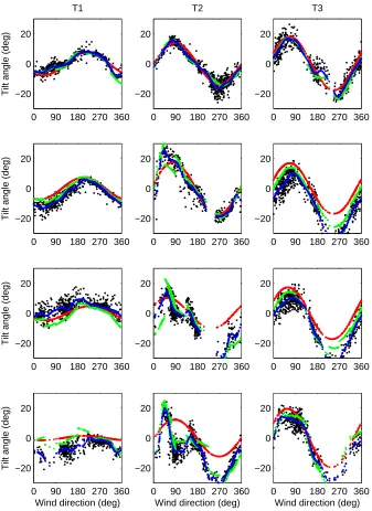
Figure 1 shows the angle of tilt, φ, from the DR method and the various planar fit methods as a function of the wind direction. Results are presented for the standard planar fit (PF) method, for the sector planar fit (SPF) method with 8 equal sectors and for the continuous planar fit (CPF) method. In fitting the functionθfor the continuous planar fitN = 4was chosen for the number of Fourier terms. In practice the first few terms dominated. Tests withN = 8did not show any improvement in the quality of the fit, and in some cases introduced spurious wiggles, particularly where there were directions with a sparsity of data. The optimal number of terms required will obviously depend on the complexities of each particular site.
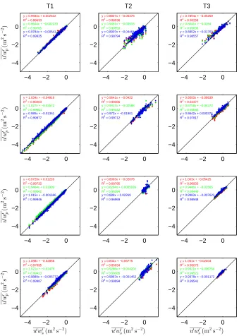
Figures 2-4 show a comparison of the fluxes calculated using the three planar fit methods (PF, SPF, CPF) against the equivalent fluxes using the DR method. Also plot-ted on the figures is a 1:1 line, and for each method the best fit equation and R2
value. Figure 2 shows the streamwise momentum fluxes,u′w′. For the planar fit methods the
direction of the streamwise velocities,u, are calculated as the 15-minute mean velocity projected onto the relevant planar surface. The effect of the different methods on cal-culating a scalar flux is demonstrated in figure 3 using the temperature fluxw′T′as an
example. Figure 4 shows results for the cross-wind momentum fluxv′w′, as previous
studies have shown this to be a quantity which is particularly sensitive to the coordinate transformation used.
av-0 90 180 270 360 −20
0 20
T1
Tilt angle (deg)
0 90 180 270 360
−20 0 20
T2
0 90 180 270 360
−20 0 20
T3
0 90 180 270 360
−20 0 20
Tilt angle (deg)
0 90 180 270 360
−20 0 20
0 90 180 270 360
−20 0 20
0 90 180 270 360
−20 0 20
Tilt angle (deg)
0 90 180 270 360
−20 0 20
0 90 180 270 360
−20 0 20
0 90 180 270 360
−20 0 20
Tilt angle (deg)
Wind direction (deg)
0 90 180 270 360
−20 0 20
Wind direction (deg)
0 90 180 270 360
−20 0 20
[image:6.595.129.466.153.616.2]Wind direction (deg)
−4 −2 0 −4
−2 0
y = 0.9594x + 0.002322 R2 = 0.99633
y = 0.9644x + −0.002233 R2 = 0.99765
y = 0.9784x + −0.00541 R2 = 0.99935
T1 u ′w ′ p (m 2s − 2)
−4 −2 0
−4 −2 0
y = 0.8827x + −0.06378 R2 = 0.98536
y = 0.9451x + −0.03918 R2 = 0.99553
y = 0.8907x + −0.04464 R2 = 0.98794
T2
−4 −2 0
−4 −2 0
y = 0.7894x + −0.05259 R2 = 0.95258
y = 0.8041x + −0.0164 R2 = 0.95836
y = 0.8802x + −0.01769 R2 = 0.98557
T3
−4 −2 0
−4 −2 0
y = 1.034x + −0.04919 R2 = 0.99203
y = 1.027x + −0.02572 R2 = 0.99664 y = 0.985x + −0.01361 R2 = 0.99977
u
′w ′(mp
2s
−
2)
−4 −2 0
−4 −2 0
y = 0.9641x + −0.0422 R2 = 0.98386
y = 0.9417x + −0.02588 R2 = 0.99442 y = 0.972x + −0.01901 R2 = 0.99712
−4 −2 0
−4 −2 0
y = 0.9593x + −0.08639 R2 = 0.84377
y = 0.8758x + −0.04372 R2 = 0.95682 y = 0.8642x + 0.003374 R2 = 0.97817
−4 −2 0
−4 −2 0
y = 0.9729x + 0.01226 R2 = 0.99732
y = 0.9464x + 0.01909 R2 = 0.99062 y = 1.015x + −0.001696 R2 = 0.99946
u ′w ′ p (m 2s − 2)
−4 −2 0
−4 −2 0
y = 0.8093x + −0.02678 R2 = 0.88785
y = 0.8204x + 0.0005939 R2 = 0.96394 y = 0.886x + 0.02269 R2 = 0.96969
−4 −2 0
−4 −2 0
y = 1.003x + −0.05425 R2 = 0.90933
y = 0.9446x + −0.02565 R2 = 0.98449 y = 0.8983x + −0.007623 R2 = 0.98948
−4 −2 0
−4 −2 0
y = 1.088x + −0.02856 R2 = 0.97095
y = 1.021x + −0.02479 R2 = 0.99413 y = 0.9889x + −0.005777 R2 = 0.99987
u ′w ′ p (m 2s − 2)
u′ws′(m2s−2)
−4 −2 0
−4 −2 0
y = 0.834x + −0.06775 R2 = 0.85934
y = 0.9286x + −0.004202 R2 = 0.99385 y = 0.9967x + −0.001452 R2 = 0.99994
u′w′s(m2s−2)
−4 −2 0
−4 −2 0
y = 1.051x + −0.02404 R2 = 0.95073
y = 0.9321x + −0.006754 R2 = 0.99521 y = 0.9378x + −0.001172 R2 = 0.99541
[image:7.595.128.467.139.615.2]u′w′s(m2s−2)
Figure 2: Momentum flux,u′w′
pcalculated using the various planar fit coordinate
sys-tems as a function of the flux in the streamwise coordinate system,u′w′
s. The different
fits are marked with different coloured dots: PF (red), SPF (green), CPF (blue). Results are plotted for towers 1, 2 and 3 (left, middle, right respectively). The black line shows the 1:1 line. Each figure shows the best fit equation and R2
−0.4 −0.2 0 0.2 −0.4
−0.2 0
0.2 y = 0.9815x + −0.001025 R2 = 0.99964
y = 0.98x + −0.001147 R2 = 0.99958 y = 0.993x + −0.001185 R2 = 0.99973
T1
w
′T ′(Kp
m
s
−
1)
−0.4 −0.2 0 0.2
−0.4 −0.2 0
0.2 y = 0.9493x + −0.003671 R2 = 0.99638
y = 0.9919x + −0.001922 R2 = 0.99887 y = 0.9525x + −0.002849 R2 = 0.99741
T2
−0.4 −0.2 0 0.2
−0.4 −0.2 0
0.2 y = 0.81x + −0.006802 R2 = 0.96264
y = 0.8259x + −0.004234 R2 = 0.96948 y = 0.8896x + −0.003979 R2 = 0.98735
T3
−0.4 −0.2 0 0.2
−0.4 −0.2 0
0.2 y = 1.052x + −0.005254 R2 = 0.98425
y = 1.044x + −0.00367 R2 = 0.99084 y = 0.9968x + −0.003307 R2 = 0.99779
w
′T ′(Kp
m
s
−
1)
−0.4 −0.2 0 0.2
−0.4 −0.2 0
0.2 y = 0.9457x + −0.002704 R2 = 0.99642
y = 0.9225x + −0.00199 R2 = 0.99379 y = 0.9351x + −0.001239 R2 = 0.99524
−0.4 −0.2 0 0.2
−0.4 −0.2 0
0.2 y = 1.019x + −0.006506 R2 = 0.94228
y = 0.925x + −0.00545 R2 = 0.9758 y = 0.8563x + −0.004073 R2 = 0.97775
−0.4 −0.2 0 0.2
−0.4 −0.2 0
0.2 y = 0.9763x + 0.0005183 R2 = 0.99865
y = 0.9628x + 0.001294 R2 = 0.99598 y = 1.02x + 0.0003599 R2 = 0.99945
w
′T ′(Kp
m
s
−
1)
−0.4 −0.2 0 0.2
−0.4 −0.2 0
0.2 y = 0.8579x + −0.001965 R2 = 0.97865
y = 0.6993x + 0.000301 R2 = 0.87477 y = 0.9006x + 0.0015 R2 = 0.98059
−0.4 −0.2 0 0.2
−0.4 −0.2 0
0.2 y = 1.078x + −0.004505 R2 = 0.95109
y = 1.01x + −0.00333 R2 = 0.98563 y = 0.9469x + −0.002312 R2 = 0.99554
−0.4 −0.2 0 0.2
−0.4 −0.2 0
0.2 y = 1.066x + −0.002366 R2 = 0.98488
y = 1.019x + −0.002054 R2 = 0.99586
y = 0.9795x + −0.0009457 R2 = 0.99953
w
′T ′(Kp
m
s
−
1)
w′T′
s(K m s−1)
−0.4 −0.2 0 0.2
−0.4 −0.2 0
0.2 y = 0.8624x + −0.004722 R2 = 0.98068
y = 0.8415x + −0.0009819 R2 = 0.96927
y = 0.9494x + −0.000406 R2 = 0.99696
w′T′
s(K m s−1)
−0.4 −0.2 0 0.2
−0.4 −0.2 0
0.2 y = 1.064x + −0.002492 R2 = 0.97755
y = 1.017x + −0.000917 R2 = 0.99766
y = 0.9958x + −0.0009575 R2 = 0.99892
w′T′
[image:8.595.125.467.181.644.2]s(K m s−1)
−2 0 2 −2
−1 0 1
2 y = 0.3743x + −0.01036R2 = 0.49377
y = 0.5883x + −0.02169 R2 = 0.73529 y = 0.5302x + −0.01557 R2 = 0.68982
T1
v
′w ′(mp
2s
−
2)
−2 0 2
−2 −1 0 1
2 y = 0.644x + −0.01354R2 = 0.85293
y = 0.6663x + −0.01751 R2 = 0.8665 y = 0.4451x + −0.009201 R2 = 0.65775
T2
−2 0 2
−2 −1 0 1
2 y = 0.4679x + −0.02537R2 = 0.71615
y = 0.5238x + −0.003414 R2 = 0.75858 y = 0.529x + 0.002493 R2 = 0.75602
T3
−2 0 2
−2 −1 0 1
2 y = 0.4676x + −0.1078R2 = 0.13869
y = 0.5661x + −0.1045 R2 = 0.28211 y = 0.5175x + −0.1096 R2 = 0.17957
v
′w ′(mp
2s
−
2)
−2 0 2
−2 −1 0 1
2 y = 0.6882x + −0.01779R2 = 0.87847
y = 0.7533x + −0.008343 R2 = 0.92764 y = 0.5631x + 0.002509 R2 = 0.78917
−2 0 2
−2 −1 0 1
2 y = 0.5728x + −0.03301R2 = 0.80901
y = 0.4848x + −0.03063 R2 = 0.73179 y = 0.4367x + −0.01239 R2 = 0.6767
−2 0 2
−2 −1 0 1
2 y = 0.7254x + −0.03774R2 = 0.824
y = 0.8644x + −0.03603 R2 = 0.90621 y = 0.9709x + −0.03849 R2 = 0.92762
v
′w ′(mp
2s
−
2)
−2 0 2
−2 −1 0 1
2 y = 0.8021x + −0.02816R2 = 0.82741
y = 0.6984x + −0.06418 R2 = 0.18937 y = 0.8293x + −0.04326 R2 = 0.63996
−2 0 2
−2 −1 0 1
2 y = 0.6079x + −0.03255R2 = 0.77822
y = 0.5188x + −0.02811 R2 = 0.72139 y = 0.5142x + −0.01464 R2 = 0.7542
−2 0 2
−2 −1 0 1
2 y = 1.165x + −0.02027R2 = 0.89875
y = 1.201x + −0.02486 R2 = 0.84905 y = 0.7584x + −0.05267 R2 = 0.8696
v
′w ′(mp
2s
−
2)
v′w′s(m2s−2)
−2 0 2
−2 −1 0 1
2 y = 0.7516x + −0.015R2 = 0.91962
y = 0.7939x + −0.009049 R2 = 0.94882 y = 0.6975x + −0.009675 R2 = 0.89511
v′w′s(m2s−2)
−2 0 2
−2 −1 0 1
2 y = 0.6516x + −0.04362R2 = 0.59445
y = 0.6017x + −0.02514 R2 = 0.75326 y = 0.5988x + −0.02197 R2 = 0.77321
[image:9.595.129.467.171.657.2]v′ws′(m2s−2)
erage wind speeds and this explains the lower scatter in the tilt angle from the double rotation (DR) method, particularly at the top of the tower. Even at the top of the tower there is evidence that the sinusoidal variation ofφwithθassumed in the standard pla-nar fit (PF) method is not necessarily accurate. Both the SPF and CPF methods show a kink inφat a wind direction of around90◦which corresponds to flow coming directly
off the nearby dense canopy. The big difference between the two methods is that the CPF deals with this smoothly while the SPF approach shows very different planar fits for the two adjacent sectors which suggests that the fit (and hence the fluxes) will de-pend in a somewhat arbitrary way on the choice of sectors. Similar large discontinuities in the SPF are observed in a number of the other plots.
Lower on tower 1 the scatter in the data increases as the wind speeds decrease and the observations become more influenced by the canopy. There is also some evidence of a bias in the scatter with the outliers being generally mostly higher or mostly lower than the average for a particular instrument. This seems unlikely physically and is possibly due to interference of the tower on the air flow. The towers are round with a diameter of about10cm and the sonic anemometers are mounted on a long boom approximately1m from the tower. The sonic anemometers have a symmetrical design with a central column so there are no preferred wind directions. These factors, together with a lack of evidence of any variation in these outliers with wind direction, suggests that it is not direct distortion of the wind flow by the tower that is the cause of this. A similar effect is observed on the other towers.
Closer to the ground, below canopy top, the impact of wind direction on the tilt becomes more pronounced. In particular the lower instruments on tower 1 show the clear benefits of the CPF approach in better representing local variations in tilt angle with wind direction. Note that both the planar fit and sector planar fit methods apply an offset correction to the vertical velocity, which in turn alters the slope of the fitted plane. This explains the offset in Fig. 1 between these methods and the tilt angle calculated from the raw data, but not the failure to capture the shape of the curve.
Towers 2 and 3 exhibit similar results, although both show a larger scatter in the data due to their more sheltered positions and lower mean wind speeds (mean wind speeds of1−2m s−1 compared to5m s−1 at the top of tower 1). The third sonic
anemometer down on tower 2 demonstrates one potential issue with the SPF method. There is very little data for wind directions of200◦to260◦. This means that the fitted
plane is not very strongly constrained in this range. The CPF deals with this data sparsity more smoothly, particularly since we only include a small number of terms in the Fourier series here. While more intelligent choices of sectors for the SPF might also help, this introduces additional complexity and subjectivity to the method.
The scatter plots of the momentum flux in Figure 2 show that for tower 1, with relatively higher wind speeds, the three planar fit methods and the double rotation into streamwise coordinates all produce very similar values foru′w′, although the
In these cases the positive fluxes are similar between the planar fit and streamwise coordinate methods.
The scatter in temperature fluxes at all three towers (Figure 3) is smaller than in the momentum fluxes, particularly within the canopy. Agreement between all four methods is generally good, with the largest differences observed at the extremes. At tower 1 there is more scatter for unstable conditions (w′T′ >0) at all heights. In the
canopy it tends to be stable conditions (w′T′<0) which leads to greater scatter. This
may be partly because stable conditions are often associated with low, variable winds and decoupled flow. In such conditions it unsurprising that there is more variability in the 15-minute flow direction compared to the planar fit. As with the momentum flux, the scatter is reduced for the CPF method compared to the PF and SPF methods.
The greatest differences between the methods are seen with the cross-wind mo-mentum fluxes (Figure 4). The low R2
values show that the 1:1 line is not a good fit to the data. There is a systematic bias at most instrument locations with all the planar fit methods showing lower fluxes than the corresponding value calculated using the streamwise coordinate rotation. The cross-wind momentum fluxes at towers 2 and 3 are larger than those at tower 1, which reflects the stronger direction wind shear with height observed in the flow separation regions at these towers (Grant et al., 2015).
The results of Lee et al. (2004) show a strong periodic directional dependence to thev′w′values which they attribute to disruption of the flow by the tower. Directional
dependence is also seen in these results (not shown), although in this case it appears to be a real effect due to differences in the surrounding terrain and canopy rather than an artifact of the tower setup. There are a couple of factors supporting this conclusion. As described above, the tower and the instrument mounts were designed to minimise flow disruption. More significantly, the instruments were mounted alternately on opposite sides of the tower. For each tower all four instruments show similar variations inv′w′
with direction, despite being mounted on different sides of the tower. If the effect was due to flow disruption by the tower it would be expected that instruments mounted on opposite sides would exhibit a different directional dependence. The evidence of physically realisticv′w′ terms suggests that applying a triple rotation to the data so v′w′ = 0would not be wise for sites with complex terrain and/or heterogeneous canopy
cover.
In common with other planar fit methods, the optimal fit for the CPF method may depend on other environmental factors including the stability, wind speed and whether the trees are in leaf. Here we have tried to minimise these effects by filtering the data, although the method could in theory be used to investigate these effects further.
alleviate this problem, but at the expense of having some larger sectors.
4
Conclusions
This paper presents an alternative to the widely used planar fit method for calculat-ing fluxes uscalculat-ing the eddy covariance method. The new continuously variable planar fit (CPF) method extends the ideas of the sector planar fit (SPF) to account for the effects of forest canopy and terrain variations with wind direction which lead to devia-tions from a simple planar fit (PF). The new method has the advantage that it does not depend on an arbitrary division of the data into different sectors, with a correspond-ing discontinuity in how the fluxes are handled at the edges of the sectors. The CPF method produces fluxes closer to those obtained with the DR method in most cases (reflecting the fact it better represents the variation in the mean streamwise deflection with wind direction), while at the same time preventing the unrealistic rotation angles and positive streamwise momentum fluxes seen with the DR method. This improved agreement with the DP method comes despite the fact that the CPF method has fewer degrees of freedom than the SPF method in this case.
One potential disadvantage of this method is that, unlike the PF method, it does not offer an estimate of the instrument offset in vertical velocity. The error estimate of the PF method assumes that the data is well represented by a planar fit and so any offset is a result of instrument error. This assumption almost certainly fails for cases with complex terrain and variable canopy cover where the CPF method is likely to be applied. This paper successfully tests the new method with data from a number of sites over complex terrain, both within and above the heterogeneous forest canopy. The comparisons are limited to momentum and heat fluxes. Further tests are required to see how the method performs for other scalar fluxes of interest, including latent heat and carbon dioxide fluxes, and the impact it has on long term cumulative fluxes.
Acknowledgements
This work was funded by the Natural Environmental Research Council (NERC) grant NE/C003691/1. ERG would like to acknowledge additional support through a NERC CASE award with Forest Research. We would also like to thank the two anonymous reviewers for some useful suggestions.
References
Dellwik, E., Bingol, F., and Mann, J., 2014. Flow distortion at a dense forest edge.
Quart. J. Roy. Meteorol. Soc.,140:676–686. doi:10.1002/qj.2155.
Dupont, S. and Patton, E. G., 2012. Influence of stability and seasonal canopy changes on micrometeorology within and above an orchard canopy: The CHATS e xperi-ment.Agric. For. Meteorol.,157:11–29. doi:10.1016/j.agrformet.2012.01.011. Finnigan, J. J., 2004. A re-evaluation of long-term flux measurement techniques
Foken, T. and Wichura, B., 1996. Tools for quality assessment of surface-based flux measurements. Agric. For. Meteorol., 78:83–105. doi:10.1016/0168-1923(95)02248-1.
Grant, E. R., 2011. Canopy-atmosphere interactions over complex terrain. Ph.D. thesis, University of Leeds, UK.
Grant, E. R., Ross, A. N., Gardiner, B. A., and Mobbs, S. D., 2015. Field observations of canopy flow over complex terrain. Boundary-Layer Meteorol.,Online First:1– 21. doi:10.1007/s10546-015-0015-y.
Lee, X., 1998. On micrometeorological observations of surface-air exchange over tall vegetation.Agric. For. Meteorol.,91:39–49. doi:i10.1016/S0168-1923(98)00071-9. Lee, X., Finnigan, J., and Paw U, K. T., 2004. Coordinate systems and flux bias error. In X. Lee, W. Massman, and B. Law, editors,A handbook of micrometeorology: A guide for surface flux measurements, pages 33–66. Kluwer academic publishers. Liu, H., Peters, G., and Foken, T., 2001. New equations for sonic temperature variance
and buoyancy heat flux with an omnidirectional sonic anemometer.Boundary-Layer Meteorol.,100:459–468. doi:10.1023/A:1019207031397.
Mammarella, I., Kolari, P., Rinne, J., Keronen, P., Pumpanen, J., and Vesala, T., 2007. Determining the contribution of vertical advection to the net ecosystem exchange at hyytiala forest, finland. Tellus B, 59:900–909. doi:10.1111/j.1600-0889.2007.00306.x.
McMillen, R. T., 1988. An eddy correlation technique with extended appli-cability to non-simple terrain. Boundary-Layer Meteorol., 43:231–245. doi: i10.1007/BF00128405.
Paw U, K. T., Baldocchi, D. D., Meyers, T. P., and Wilson, K. B., 2000. Correction of eddy-covariance measurements incorporating both advective effects and density fluxes. Boundary-Layer Meteorol.,97:487–511. doi:10.1023/A:1002786702909. Turnipseed, A. A., Anderson, D. E., Blanken, P. D., Baugh, W. M., and Monson, R. K.,
2003. Airflows and turbulent flux measurements in mountainous terrain. Part 1. Canopy and local effects. Agric. For. Meteorol., 119:1–21. doi:10.1016/S0168-1923(03)00136-9.
Wilczak, J. M., Oncley, S. P., and Stage, S. A., 2001. Sonic anemome-ter tilt correction algorithms. Boundary-Layer Meteorol., 99:127–150. doi: 10.1023/A:1018966204465.
Yuan, R., Kang, M., Park, S.-B., Hong, J., Lee, D., and Kim, J., 2011. Expansion of the planar-fit method to estimate flux over complex terrain. Meteorol. Atmos. Phys.,