This is a repository copy of A travel time-based variable grid approach for an activity-based cellular automata model.
White Rose Research Online URL for this paper: http://eprints.whiterose.ac.uk/124167/
Version: Accepted Version
Article:
Crols, T orcid.org/0000-0002-9379-7770, White, R, Uljee, I et al. (3 more authors) (2015) A travel time-based variable grid approach for an activity-based cellular automata model. International Journal of Geographical Information Science, 29 (10). pp. 1757-1781. ISSN 1365-8816
https://doi.org/10.1080/13658816.2015.1047838
© 2015 Taylor & Francis This is an Accepted Manuscript of an article published by Taylor & Francis in International Journal of Geographical Information Science on 27/05/15,
available online: http://www.tandfonline.com/10.1080/13658816.2015.1047838
[email protected] https://eprints.whiterose.ac.uk/ Reuse
Items deposited in White Rose Research Online are protected by copyright, with all rights reserved unless indicated otherwise. They may be downloaded and/or printed for private study, or other acts as permitted by national copyright laws. The publisher or other rights holders may allow further reproduction and re-use of the full text version. This is indicated by the licence information on the White Rose Research Online record for the item.
Takedown
If you consider content in White Rose Research Online to be in breach of UK law, please notify us by
A travel time-based variable grid approach for an activity-based
cellular automata model
Tomas Crols
a,b*, Roger White
c, Inge Uljee
b, Guy Engelen
b, Lien Poelmans
band Frank Canters
aaCartography and GIS Research Group, Department of Geography, Vrije Universiteit
Brussel, Brussels, Belgium; bEnvironmental Modelling Unit, VITO – Flemish Institute for Technological Research, Mol, Belgium; cDepartment of Geography, Memorial
University of Newfoundland, St. John’s, NL, Canada
*Corresponding author. Address: Vrije Universiteit Brussel, Department of Geography,
Pleinlaan 2, 1050 Brussel, Belgium. Phone: +3214336758 or +3226293783. E-mail:
This is an Accepted Manuscript of an article published by Taylor & Francis
Group in the International Journal of Geographical Research on 27/05/2015,
A travel time-based variable grid approach for an activity-based
cellular automata model
Urban growth and population growth are used in numerous models to determine
their potential impacts on both the natural and the socio-economic systems.
Cellular automata (CA) land-use models became popular for urban growth
modelling since they predict spatial interactions between different land uses in an
explicit and straightforward manner. A common deficiency of land-use models is
that they only deal with abstract categories, while in reality several activities are
often hosted at one location (e.g. population, employment, agricultural yield,
nature…). Recently, a multiple activity-based variable grid CA model was proposed to represent several urban activities (population and economic activities)
within single model cells. The distance-decay influence rules of the model included
both short- and long-distance interactions, but all distances between cells were
simply Euclidean distances. The geometry of the real transportation system, as well
as its interrelations with the evolving activities, were therefore not taken into
account. To improve this particular model, we make the influence rules functions
of time travelled on the transportation system. Specifically, the new algorithm
computes and stores all travel times needed for the variable grid CA. This approach
provides fast run times, and it has a higher resolution and more easily modified
parameters than the alternative approach of coupling the activity based CA model
to an external transportation model. This paper presents results from one Euclidean
scenario and four different transport network scenarios to show the effects on
land-use and activity change in an application to Belgium. The approach can add value
to urban scenario analysis and the development of transport- and activity-related
spatial indicators, and constitutes a general improvement of the activity based CA
model.
Keywords: cellular automata; activity-based modelling; land-use change; urban
growth; multimodal transportation networks
1. Introduction
Population growth and urbanisation put increasing pressure on both natural resources and
the quality of the urban environment. This phenomenon occurs predominantly in rapidly
spatial planning history (Ravetz et al. 2013). Therefore, urban modelling continues to be
a key research topic not only at the global scale (Lambin and Geist 2006), but also at the
regional scale in land-use modelling (e.g. Barredo et al. 2003, de Kok et al. 2012), and in
all sorts of environmental studies (e.g. Geertman and Stillwell 2009, Van Steertegem et
al. 2009, Hansen 2010).
Many types of models have been developed (Batty 2005, Haase and Schwarz
2009), including land-use and transport interaction (LUTI) models (Wegener 2004,
Chang 2006, Iacono et al. 2008), multi-agent systems (MAS) (Bura et al. 1996, Parker et
al. 2003, Matthews et al. 2007, Gilbert 2008) and cellular automata (CA) models. CA
models have become popular for studies of land-use change in urbanised areas because
of their simplicity and flexibility (Santé et al. 2010) and their ability to simulate realistic
urban patterns by incorporating path dependence and self-organisation (Poelmans and
Van Rompaey 2010). Recent applications include Engelen et al. (2007), Almeida et al.
(2008), Stanilov and Batty (2011), de Kok et al. (2012), Aljoufie et al. (2013), and
Fuglsang et al. (2013).
Most urban models, including CA models, focus on the rather abstract and
categorical concept of land-use change. Each unit is in one dominant land-use state at
each time step in the simulation interval. However, in the real world, many urban zones
are characterised by mixed land uses (e.g. residential and commercial functions). In
regions with extensive urban sprawl, like Flanders, Belgium, where ribbon development
is common, urban and non-urban functions also become mixed, turning agricultural and
natural areas into highly fragmented landscapes (Poelmans and Van Rompaey 2009).
MAS capture the interaction between different types of activities in a direct way, but need
a huge amount of data to realistically represent the agents and their spatial behaviour
simulations on large study areas, which can only be solved by aggregating agents into
‘super-individuals’ and resorting to parallel computing (Parry and Bithell 2012). A more
straightforward solution for this is to introduce activities and their interactions into the
simple but efficient grid structure of a CA model. Then a list of all activities that are
present in each cell of the model provides an appropriate description of the complexity of
land use in both dense urban areas and regions with urban sprawl.
Urban CA models rely in the first place on distance-dependent interactions among
land uses to predict the future development of urban regions. These are captured in the
neighbourhood effect. The neighbourhood effect is calculated by means of influence
functions that define the effect of each cell in the neighbourhood on the cell for which the
neighbourhood effect is being calculated — i.e. the focal cell — where that effect depends
on both the distance and the state of the cell. The contributions of all cells in the
neighbourhood are summed to get the neighbourhood effect on the focal cell. A
neighbourhood effect is calculated for each possible state that the focal cell could have.
Traditionally, neighbourhoods are small and only capture short-distance effects up to a
maximum of 1 km. Some modellers tackle this problem by coupling the CA component
to a regional gravity-based spatial interaction model of the economy and population (e.g.
Engelen et al. 1995, White and Engelen 2000, Engelen et al. 2007, Lauf et al. 2012).
However, the coupling of such a macro model with a CA model has several
disadvantages: additional parameters are needed to link the models, the regions may be
large but each is represented by a single point, typically the centroid, not all levels of
spatial interaction are represented, and finally it is still impossible to have several
activities in a single CA cell (White et al. 2012). A solution is to change the topology of
the CA model, which has an influence on its dynamics (Baetens et al. 2013), so that
Andersson et al. (2002a, 2002b) introduced a variable grid representation of the
cell neighbourhood in order to make it computationally feasible to expand the
neighbourhood to include the entire modelled area, so that all cells could have an effect
on the possible land use of each individual cell. White (2006) extended the variable grid
approach by including activities in it: both land uses and their associated activities are
represented and forecasted for each individual cell. For the purpose of calculating the
neighbourhood effect, cells, and their associated land uses and activities, are aggregated
into increasingly large supercells the greater the distance from the focal cell. The
expansion factor is three, which gives a set of nested Moore neighbourhoods. In other
words, supercells consist of 32L unit cells and have a resolution of 3L times the resolution
of the modelling grid, where L, an integer, is the level number of the variable grid (Figure
1). In the cell neighbourhood, only the cells belonging to the immediate Moore
neighbourhood (L = 0) have the unit cell resolution. This approach keeps calculations fast
and simple.
[Figure 1 about here]
Other work further developed these concepts: van Vliet et al. (2009) discuss the
use of a variable grid approach for land-use change only, van Vliet et al. (2012) tested an
activity-based model without a variable grid, while White et al. (2011) applied the full
approach to the Dublin region. In van Vliet et al. (2012) and White et al. (2011), only one
activity type is considered in each cell, consistent with the dominant land use. White et
al. (2012) introduced a multiple-activity CA model that can really deal with
multifunctional land use, where each cell has values for all activity types considered in
the model. Initial results obtained with this model seem promising, yet some challenges
remain unsolved. One striking simplification in all variable grid approaches proposed to
with a size of sometimes several hundred kilometres instead of travel times generated by
a transport model component.
Many studies have shown that transport and land use are strongly interrelated
systems, but the nature of the relation is often debated. Both the road system and the
public transport system influence and are influenced by the land-use characteristics of
urban areas and their related activity patterns. The standard work of Newman and
Kenworthy (1989) suggested a negative relationship between population density and
energy use in transportation. Although this work has been criticised as being simplistic
(van de Coevering and Schwanen 2006), other authors have also found statistical
relationships between the urban structure, activities, access to public transport and
commuting patterns (e.g. Sohn 2005, Schwanen and Mokhtarian 2005, Næss 2010,
Fuglsang et al. 2011). Attitudes (e.g. Handy et al. 2005) as well as socio-economic
characteristics of a country or region, such as income and fuel prices (Giuliano and
Dargay 2006), have also been found to be important. Hansen (2009) used a raster-based
approach to show that many new residential and industrial areas in Northern Denmark
have high accessibility to existing towns, and for industry also to motorway exits. In
regions with much sprawl, however, it is almost impossible to build a public transport
network with a high competitiveness and efficiency; nevertheless, public transport can
influence dynamics within and between city centres (Camagni et al. 2002). The reality is
without any doubt complex, and to some degree specific to countries or regions.
Over the past decades, a considerable number of LUTI models have been
developed. According to Wegener (2004), most of these models describe the link between
slowly changing systems (land use, networks and buildings), fast changing systems
(activities) and immediate changes (transport as such). Hagen-Zanker (2012) compared
— in particular MEPLAN (see e.g. Echenique 2004) and UrbanSim (Waddell 2002). He
concluded that although these three modelling strategies are fundamentally and
computationally different, all of them may lead to similar results if their weaknesses are
overcome. Unlike LUTI models, most CA models do not have an intrinsic economic or
transport component. An activity-based model includes economic activities, but should
still be improved by taking transport into account.
Some LUTI models are linked to a stand-alone transport model, others have their
own transport subsystem. Aljoufie et al. (2013) coupled a CA-based land-use model,
developed with the Metronamica framework and thus based on the work of White et al.
(1997), to a stand-alone transport model for the city of Jeddah. The resulting generalised
cost of the transport model is used as an input for the accessibility component of the
land-use model. Nevertheless, the accessibility component does not directly influence the
distance between cells in the influence rules. Blečić et al. (2011) incorporated distance
effects directly into their CA model. They represented the short-distance CA
neighbourhood effect and a long-distance accessibility effect separately in what they call
a ‘wave model’. Two different signals of land-use influences are propagated between
cells to simulate vicinity and accessibility. Vicinity is here represented by a
small-neighbourhood Euclidean influence function. Accessibility is modelled as an influence
signal that gets weaker with increasing distance.
In this study, we use the model of White et al. (2012) to test how travel times can
be integrated into the variable grid neighbourhood rules (except for the close
neighbourhood) and show how this impacts modelling results. We define different
transport network scenarios to compute these travel times with a road-based or a
multimodal network. The remainder of the paper starts with a short description of the
methodology to define travel time-based distances for the influence rules of the model.
In section 4, we apply this methodology to the case of Belgium, and define a ‘Euclidean
scenario’ and four ‘network scenarios’. In section 5, we compare the results obtained with
the various transport scenarios. This is followed by a discussion in section 6, including
suggestions for future research, and a short conclusion in section 7.
2. A multiple activity-based variable grid cellular automaton
The modelling approach proposed by White et al. (2012) constitutes a multiple
activity-based cellular automaton. It makes use of active, passive and static land uses. Active land
uses change directly as a result of CA dynamics as forced by exogenous demands: these
are land uses such as residential, industrial or commercial. Passive land uses, such as
various agricultural or natural land-cover states, change as a consequence of the dynamics
of the active land uses — they are taken over or abandoned by active land uses. Static
land uses, like water and parks, cannot change state and are not subject to the CA
dynamics, though may affect it. By definition, there exists a one-to-one relationship in
the model between active land-use types and activity types. In an active land-use cell,
primary activities are defined as those associated with the dominant land use (e.g.
population in residential land use). However, each cell can also have non-zero values for
activities that are primarily associated with other land uses (e.g. employment in residential
land use). Such activity is referred to as secondary activity. Passive and static land-use
categories have no associated primary activity, but may host secondary activities; for
example, agriculture cells may have a resident population.
Several factors are incorporated in the model to determine future activity values,
with the neighbourhood effect being the most important one. Within the variable grid
approach this effect contains the influence on a cell of all activities throughout the entire
the neighbourhood effect is being calculated, and the centroid of one of its variable grid
neighbour cells j can only have specific discrete rook or bishop values since the resolution
of variable grid cells increases by a factor of 3 for each level. Therefore dij can only be R,
R, 3R, 3 R, etc., with R being the resolution of the CA grid — i.e. the size of a unit
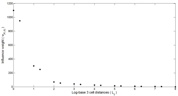
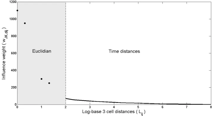
cell in the grid. Next, the weights W of the influence functions (Figure 2) are expressed
in the model as functions of log-base 3 cell distances Lij:
Lij = log3(dij/R) (1)
WJK,dij = fJK (Lij) (2)
where WJK,dij is the weight given by the influence function fJK for the influence of activity
J on activity K at distance dij. The possible rook or bishop values of Lij are then 0, 0.315,
1, 1.315, etc.
[Figure 2 about here]
The activity potential VKi for an activity K on a cell i for the next time step is
calculated as:
VKi = r ZKi XKi SKi NKi (3)
where r is a random perturbation term, ZKi is the zoning status for activity K on cell i, XKi
is a measure of accessibility to the transport network for activity K on cell i, SKi is the
suitability of cell i for activity K, and NKi is the neighbourhood effect. The random
perturbation, which is necessary to account for the possible differences in actor behaviour,
is drawn from a highly skewed distribution, so that most perturbations are very small. A
fixed seed is used in the random generator to make different scenarios comparable. The
NKi = J j WJK,dij (AJj / AJ) (4)
where AJj is the total activity J on cell j, and AJ is the total activity J in the study area.
Next, the land-use transition potential VTKi for the associated active land use UK
on cell i is calculated as:
VTKi = DKi (VKi)mK + IK (5)
where DKi is a factor representing diseconomies of agglomeration, accounting for the
effect of congestion and high land prices on location decisions, mK is a parameter to be
calibrated for each activity K, and IK is the inertia value for activity K, representing the
tendency of land uses and activities to remain fixed because of relocation costs. Cells are
ranked based on their largest land-use transition potential, and subsequently get the land
use for which they have the highest potential until the number of cells demanded by the
input scenario for each land use UK is met.
The input scenario also defines the total amount of activity K to be located at each
time step. A parameter QK determines the proportion to be distributed as primary activity
on the associated land use UK. The allocation of primary activity to the cells with the
associated land use is in proportion to the activity potential VKi. The remainder of activity
K is distributed to cells of the other land uses as secondary activity on the basis of activity
potentials, as modified by compatibility factors representing the compatibility of activity
K with the various land uses. Several rescaling operations are necessary to keep all
activity totals and proportions consistent. For a full description of the model, the reader
is referred to White et al. (2012).
3. Travel time computations within the Variable Grid CA
activity-based variable grid CA model divide naturally into two parts: an inner zone with
a radius of approximately 1 km, where the influence weights decrease rapidly with
increasing distance, and the rest of the study area, where the weights decrease slowly as
a function of distance. This can be seen in Figure 2. Therefore, in incorporating
network-based distances in the activity-network-based CA model, we decided to deal with the immediate
neighbourhood of a location and more distant areas in different ways. In our approach,
the classic Euclidean concept of vicinity still holds for distances within the range of a
local CA neighbourhood of approximately 1 km radius, as used in the MOLAND
modelling framework (Engelen et al. 2007). For long-distance interactions, however, we
introduce time distances through the network. To make this dual approach compatible
with the variable grid, the point at which the transition between Euclidean and network
distances occurs needs to be between two levels of the variable grid. The level at which
the network distances are introduced will be referred to as the network grid level or level
LNG.
This approach, tailored to the specific requirements of the variable grid CA, is
more effective than the alternative of coupling the variable grid CA to a transportation
model to provide the required travel time distances. It can offer higher resolution than a
typical transport model and thus more accurate distances, while requiring fewer distances
to be stored in memory. As an internal algorithm it gives fast run times if updates are
desired during the simulation, or if the modeller wants to execute a full model calibration,
including transport-related parameters.
Nevertheless, calculating travel times and simulating travel behaviour between a
number of widely separated points involves a reasonable amount of computation time.
For polygon-based modelling approaches, adaptive zoning can be an alternative approach
thereby develops a new zone map for each origin with small zones nearby and larger
zones further away, based on the idea that exact locations are less important for
long-distance interactions. Essentially, the same reasoning lies at the basis of the variable grid
approach. Some studies have even investigated whether network distances, represented
by a weighted lp norm, are just mathematical functions of Euclidean distances (e.g. Berens
1988, Brimberg et al. 2007). Although these studies led to interesting results for some
regions, especially for cities with rectangular road patterns, we believe that these results
are not relevant to our model, which must be applicable to a wide variety of network
configurations.
Therefore, we define a fixed grid zone system that consists of supercells of a
specific level, LNG, but unlike the template of supercells in the variable grid itself, it is not
displaced as we move from one unit cell to another. We call this the network grid, or NG,
and its cells the network grid cells, or NG cells. It has resolution RNG = 3LNG R, where R
is the resolution of the unit cell grid. Note that the resolution RNG is equal to the size of
the immediate neighbourhood in which the Euclidean distance calculation is applied.
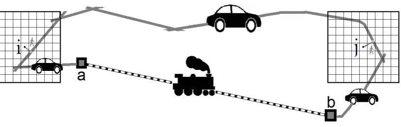
The network time distance between a unit (L = 0) cell within a fixed NG cell and
the centroid of a distant supercell (L ≥ LNG) is then taken to be the network distance
between the centroid of the NG cell containing the unit cell and the centroid of the NG
cell containing the centroid of the supercell (Figure 3). We call the NG cell containing
the unit cell the origin of the transport computation, and we call the NG cell containing
the centroid of the supercell the destination. As already indicated, we only have to store
network distances between specific needed combinations of NG cells. The only needed
‘destinations’ for an ‘origin’ NG cell are exactly the centroids of all the variable grid
neighbour cells of the central unit cell of an NG cell with L ≥ LNG. Therefore, the results
directions (top, top right…), Lmax is the highest needed level number of the variable grid,
and NNG is the total number of NG cells. The storage size is significantly smaller than a
NNG x NNG matrix, since the value of Lmax is, even for large regions, often only 6 or 7.
[Figure 3 about here]
Some supercells will lie partly outside the area being modelled. Since it does not
make sense to calculate distances to points outside the study area, an algorithm was
developed to determine the centroid of that part of the supercell that is within the study
area. The NG cell containing that centroid is then used to determine the network distance.
For the sake of generality and realism the network used to calculate travel times
can be a multimodal one. The one used here has two components: the road network, and
public transport — specifically rail in the current application (Figure 4). Both components
can be combined to generate weighted time distances, or one specific component can be
selected. If roads only are used, the weights are respectively 1 and 0. For public transport,
however, displacements are always multimodal since the road network must in general
be used to reach a station. These access times by road are calculated with the road network
component. Finally, a Euclidean displacement corresponding to a low speed, which we
call the Euclidean speed, is added to reach the nearest point in the road network. Note
that this Euclidean travel time is treated as part of the network distance. To this are added
the Euclidean travel times from the origin unit cell to the centroid of the origin NG cell,
and from the centroid of the destination NG cell to the centroid of the destination variable
grid supercell. The road network itself has known speeds for all road segments, while the
public transport network is characterized by an origin-destination travel time matrix, with
the origins and destinations being stations on the network.
In the road network component, we calculate network travel times with the
shortest path algorithm of Dijkstra (1959), applied to all needed origins. We verify
whether travelling on a straight line between the two NG centroids at low speed — the
‘Euclidean speed’ — is indeed slower than travelling to and then through the network.
This verification is especially important in cases where the road network consists of major
roads only, and the Euclidean distance can be used to represent a more direct route using
minor roads that are not included in the network.
The public transport component is mainly designed for rail travel but can also be
used for local public transport. In either case, the calculation of effective travel times
through the network requires data on (1) average travel time, and (2) frequency of service
between each pair of stations on the network. Frequency of service is defined as the total
number of possible connections between the stations per hour, either direct or indirect,
but earlier departures should not result in later arrivals. The frequency is used to add a
penalty to the average travel time, where the penalty is inversely proportional to the
frequency. Finally, the road network travel times to reach the stations from the origin and
destination centroids in the network grid are added. Thus the multimodal travel time is
given by:
tm,ij = tp,ab + C / fab + tr,ia + tr,bj (6)
where tm,ij is the multimodal transport time between two NG cells i and j, tp,ab is the
average public transport travel time between the departure station a and the arrival station
b, C is the frequency penalty parameter, fab is the frequency of service between stations a
and b, tr,ia is the road travel time from the origin NG cell i to the departure station a, and
tr,bj is the road travel time from the arrival station b to the destination NG cell j.
As already indicated, the travel time distance is a weighted average of the various
possibility of giving more weight to the fastest mode with the introduction of a parameter
F. If F > 0, then it will increase the weight of the fastest mode between two NG cells, and
decrease the weight of the slowest mode. Hence, the parameter introduces the option of
developing scenarios where the existence of one fast travel mode between certain
locations suffices to make the associated cells relatively more attractive for activities. The
weighted network time tij between NG cells i and j is then calculated as follows:
tij = tm,ij
+ tr,ij (7)
where tm,ij is the multimodal network time between i and j, tr,ij the road network time
between i and j, wm the multimodal weight, and wr the road weight (with wr = 1 – wm).
The public transport component is fully optional: by choosing wm = 0, only the road
network is used. If wr = 0, then travelling by road towards stations is still possible, but a
straight displacement at low ‘Euclidean speed’ is used when no station is located near one
of the NG cells. This is of course a rather theoretical option to test the abilities of the
model. The maximum road distance to reach a station can be specified, and it can be
different for major and minor stations. A nearby major station overrides a minor one,
except in a specified smaller zone around the minor station.
Travelling via a multimodal network is often slower than travelling by road, thus
tij is often larger than tr,ij, which would have an illogical effect on activity potentials of
cells close to stations. Therefore, when wm and wr are between 0 and 1, equation (7) is
only used to calculate the weighted travel time for combinations of NG cells where both
cells are close to a station. For all other combinations of cells, the calculated road time is
penalised proportionally to the importance of multimodal travelling:
tij =
where P ≥ 1 is a parameter that defines how much the road time has to be penalised: the
smaller the value of P, the larger the increase of the road time.
The final time distance tij can subsequently be used as an input to determine the
weights in the influence functions of the CA neighbourhood effect, except for the close
neighbourhood where distances are still Euclidean. This division between the close and
the far neighbourhoods generates a continuity problem. The weights of the influence
functions are dependent on log-base 3 cell distances, as specified by equations (1) and
(2). The distance dij of equation (1) is still Euclidean if it is shorter than RNG. For the
longer distances, we obviously have to convert the travel time tij into a relative distance
dij that is comparable with Euclidean distances since we do not want influence functions
that are in two different intervals dependent on two different quantities. Because the
influence weights are values that have to be calibrated for each possible cell distance, it
makes sense to work with a continuous range of cell distances. Consequently, we set the
shortest calculated travel time between any unit cell in the modelling area and one of its
variable grid neighbours equal to the network grid resolution RNG, since RNG is the upper
boundary of the range of Euclidean distances. Next, all the other travel times are scaled
proportionally as follows:
dij = tij (RNG / ts) (9)
where dij is the relative network distance between NG cells i and j, tij the calculated
network travel time between i and j, RNG the resolution of the network grid NG, and ts the
shortest calculated network travel time in the study area. Finally, all distances are
converted with equation (1) to be expressed in logarithmic cell distances L, so that these
cell distances can be used to find the corresponding neighbourhood influence weights
from equation (2). For the short Euclidean distances (L < LNG), L can only have Euclidean
any value of L is possible. An example of a mixed Euclidean distance-decay and time
distance-decay influence function can be seen in Figure 5.
[Figure 5 about here]
4. Study area and implementation
This study is a continuation of the work of White et al. (2012), which focused on the
Belgian case. Hence, in this study too, we applied and tested the adapted activity-based
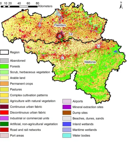
CA model to Belgium (map: see Figure 6). Several studies have discussed the problem
of urban sprawl in Belgium (e.g. Poelmans and Van Rompaey 2009, De Decker 2011)
and the link between urban land use and the transport network (e.g. Vandenbulcke et al.
2009, Boussauw et al. 2012). Low land prices together with the dense road network in
the northern part of Belgium have led to large areas of urban sprawl, and more specifically
ribbon development along the roads (Antrop 2000). Meanwhile, the average commuting
distance continues to increase because the population growth in many peri-urban
municipalities is much higher than the growth of jobs, while the opposite is true for cities
(Boussauw et al. 2011).
[Figure 6 about here]
Studies of both home-to-work travel and general travel in Belgium indicate that
individual car travel is far more common than any other transport mode (Thys and
Andries 2011, Vandenbulcke et al. 2009). A survey by the Belgian Federal Department
of Transport and Mobility indicates that 67% of Belgian employees commute individually
by car. Train travel is the second most used mode with 9.5%. It is especially popular for
long distances (> 30 km) and for travel to large cities (Thys and Andries 2011). Thus, a
in a realistic way, yet train travel towards the most important stations can improve the
model significantly. As local public transport, mostly by bus, is less popular except in
some cities, we have not yet included it in our analysis. Hence, we compare five different
scenarios for determining distance: (1) the Euclidean distance approach of White et al.
(2012); (2) road-based network distances; (3) a ‘congestion’ scenario, which uses
road-based network distances with congestion effects in the central area of Belgium; (4) a
rather theoretical ‘train only’ scenario with multimodal weight wm = 1, which means that
Euclidean paths with low speeds are used when train travel is not possible; and (5) a
‘choice’ scenario with road weight wr = 0.7, and multimodal weight wm = 0.3.
Road data come from the NAVSTREETS database for Belgium, the Netherlands
and northern France, made available by the Flanders Geographical Information Agency,
AGIV. We exclude the least important local roads (functional class 5) and estimate
average speeds on the basis of legal maximum speeds for all road segments as provided
in the database (Table 1). The ‘Euclidean speed’ is given a low value of 5 km/h. The
‘congestion’ scenario is largely based on a report of the Flemish Traffic Study Centre
(Vlaams Verkeerscentrum: Hoornaert et al. 2014). It generally assumes lower speeds in
the central area of Flanders between Ghent, Antwerp, Brussels and Leuven, and lower
motorway segment speeds based on saturation statistics.
[Table 1 about here]
An origin-destination train time matrix could not be provided by the Belgian
National Railway Company (NMBS/SNCB); therefore we reconstructed it from their
website for the most important origin-destination pairs. The resulting matrix contains
average travel time and frequencies per hour for weekday connections in 2013, between
the 18 largest major stations (> 8000 users per weekday in 2009) and all 116 stations
to start model runs from the year 2000, since there were no major changes in the train
schedule during the period 2000-2013. All missing links are handled as origin-destination
pairs where travel by train is not possible. Since train commuting is mainly towards the
big cities, we believe that this limited matrix covers the vast majority of the important
train connections for a land-use model. After initial tests, and following observations by
Thys and Andries (2011), we used a maximum distance of 10 km for the access and egress
legs by car to and from train stations in multimodal travelling. A major station overrides
a minor one except in the NG cell of the minor station itself.
Land-use data come from the Corine land-use / land-cover data set for 2000,
which was aggregated to a 300 m grid (Figure 6). Activity maps for population and
employment were reused from White et al. (2012). There are three urban categories in
the Corine map that were associated with primary activities: the discontinuous urban
fabric (associated with population), the continuous urban fabric (associated with ‘urban’
employment: wholesale, retail, hotels and catering, and finance), and industrial or
commercial units (associated with all other employment). As our main aim is to assess
the impact of different transport scenarios on the model outcome, and compare the results
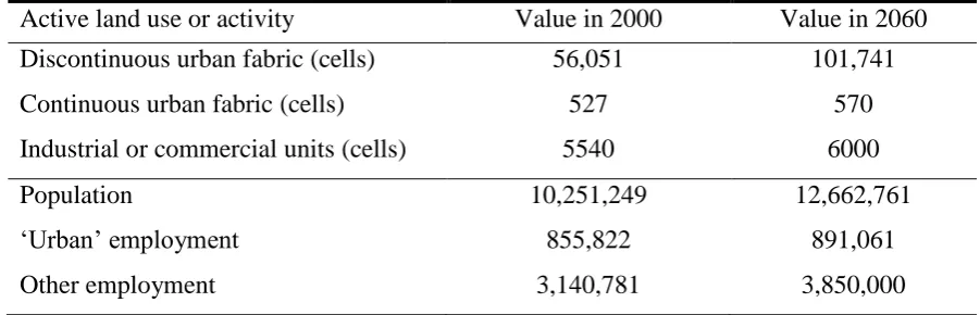
that are obtained with a simple Euclidean scenario, we ran simulations from 2000 to 2060
with the same parameters, rules, land-use area changes, and population and employment
growth (Table 2) as those used in White et al. (2012), even though that paper indicated
that this growth is somewhat excessive, especially for the discontinuous urban land use.
However, a large land-use growth helps to visualise transport scenario differences.
Since the modelling resolution is 300 m, we could have used LNG = 1 so that the
boundary between Euclidean and network travel would be 900 m, which is close to the
‘ideal’ boundary of 1 km. However, in order to keep the computation time reasonable for
settings and with a 64-bit version of the software, the calculation of all needed network
distances takes +/- 10 min on an Intel® Core™ i5-2520M CPU. Using another distance
algorithm could still reduce the run time. The network distance calculations are normally
only performed once; if the network or link speeds do not change between simulations
the calculations do not need to be repeated. The land use and activity calculations take
approximately 2 min for 15 years of simulation without updating the network distances.
The program uses about 500 MB of RAM memory.
Initial tests were done to determine suitable values for the parameters C, F and P
in equations (6), (7) and (8). We chose C = 20 min, F = 5 and P = 2, yet these choices
proved to have only a limited influence on the model results. Only for extreme values, or
when the parameters are omitted (C = 0 min, F = 0, P + ∞) do the results differ
significantly: yet, even then, differences are still slightly smaller than between the
transport scenarios (at most, about 500 cells have a different land use; most population
differences are below 1 person/km²).
[Table 2 about here]
5. Results
Land use and activities were modelled for the five transport scenarios for 2000 to 2060.
To make the comparison of the resulting land-use and activity patterns of the alternative
transport scenarios easier, we defined an accessibility index to produce maps of the effort
needed to travel from each network grid cell towards the centroids of its variable grid
neighbours in a specific transport scenario. For the network scenarios, we first calculate
two sums: (1) the sum of all possible network times tij from an origin NG cell i to all the
NG cells j containing the centroids of its variable grid neighbours, and (2) the sum of the
network and Euclidean distance sums. The very long distances towards the high-level
variable grid neighbours (L ≥ 5) were not included in the index to avoid boundary effects.
Moreover, the neighbourhood effect weights for these levels are very small. To arrive at
a standardised index, we replace the smallest value in the study area by 1: this is the most
accessible NG cell. All larger values (less accessible NG cells) are scaled proportionally.
The results for the four network scenarios can be seen in Figure 7.
[Figure 7 about here]
In the ‘road-based’ scenario, the north of Belgium has the best accessibility
values, especially in the large cities and along the motorways (Figure 7a). The
‘congestion’ scenario produces a rather different pattern, with lower accessibility values
in the central part of Flanders and around Brussels (Figure 7b); the best values are now
situated along the motorways west and south of this region. The ‘train only’ scenario has
a very distinct accessibility map with the best accessibility values around the most
important stations, especially around Brussels (Figure 7c). The accessibility map of the
multimodal scenario has a fairly similar pattern to that of the ‘road-based’ scenario, but
logically, values are clearly worse where there is no major station nearby (Figure 7d).
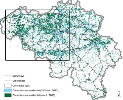
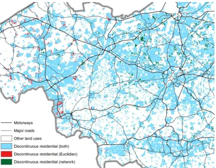
In general, the predicted land-use change patterns between 2000 and 2060 are
rather similar for all the network scenarios. The discontinuous residential area grows
significantly in the central area of Flanders between Brussels, Antwerp and Ghent, as well
as in the southwest of Flanders. This is shown for the ‘road-based’ scenario in Figure 8.
The differences between the ‘road-based’ and most other scenarios are distinct but less
pronounced than the overall growth pattern in all scenarios (Figures 9, 11, 13). The
differences between the scenarios stand out more strongly in the activity values,
[Figure 8 about here]
In the road network-based model the urban growth in the central areas is slightly
higher in 2060 than in the Euclidean model and vice versa for the peripheral areas (Figure
9). Most interestingly, some of the more accessible cells in the peripheral areas also
become residential. Although the general pattern in the population difference map is
harder to discern, the population values are somewhat higher next to major roads as well
as in the centres of the major cities (Figure 10).
[Figure 9 about here]
[Figure 10 about here]
The residential land-use difference map between the scenarios without and with
congestion clearly shows that the model is sensitive to network speed differences (Figure
11). The population growth is also smaller in the suburban regions of central Belgium in
this ‘congestion’ scenario (Figure 12). The ‘train only’ scenario leads to some remarkable
but logical differences, with much more residential growth in central areas that are more
accessible to rail stations (Figure 13). The differences in population compared with the
‘road-based’ scenario show a reasonable pattern with more population not only in the
‘train only’ scenario in big cities but also around smaller stations with good connections
to big cities. Rural areas, as well as some areas near smaller stations lacking good
connections with the centre of Belgium (e.g. in West Flanders), gain less population
(Figure 14). The ‘choice’ scenario produces growth patterns similar to those of the ‘
road-based’ scenario. Only some slight differences can be noted, such as somewhat higher
population values in big cities.
[Figure 11 about here]
[Figure 13 about here]
[Figure 14 about here]
6. Discussion
The transport component of the activity based CA model discussed in this paper is a
useful extension of the original version of White et al. (2012) for studying the influence
of existing and evolving transport networks on land-use dynamics. The accessibility
measure used in the original model, XKi in equation (3), was based on a weighted
Euclidean distance to reach the network from a cell, and thus represented only a cell’s
accessibility to the transport network, rather than its general accessibility to the region.
The new model individually computes the anisotropic accessibility of a unit cell towards
its supercells and saves it in a structure adapted to the variable grid. The structure of the
distance grid is more independent of urban development than a population-based zone
system, as often used in transport models (e.g. the model of the Flemish Traffic Study
Centre). This is an advantage in less-populated areas, which are important for future
development, but can be a disadvantage in current urban areas. Nevertheless, more
detailed zones are possible in our model with a lower network grid level LNG. Moreover,
we define useful parameters to enhance an easy definition of long-term transport
scenarios with different modes within an activity and land-use modelling context.
The transport scenarios indeed generate different results, both in terms of land use
and activity patterns. The ‘congestion’ and the ‘train only’ scenarios lead to pronounced
differences compared with the ‘road-based’ scenario. In places where the value of the
accessibility index is clearly higher for the ‘congestion’ scenario (worse accessibility),
less land is converted to urban land uses, and the population growth is significantly
smaller (Table 3). Cells that have slightly worse accessibility in the central areas seem to
growth were fixed, and other mechanisms in the model normally produce the largest
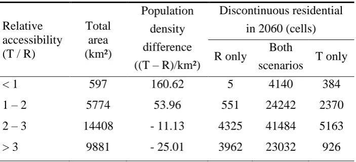
growth in those central areas. The same conclusions largely hold for the ‘train only’
scenario in comparison with the ‘road-based’ scenario (Table 4). The best locations in the
‘train only’ scenario are those close to large stations, and those are often already built-up.
New space for urban development is limited. Nevertheless, the model predicts substantial
densification, since almost 100,000 extra people (or 160 per km²) are allocated to these
areas, compared to the ‘road-based’ scenario. The regions around these areas also gain
extra residential land use and population, while there is clearly less growth in remote
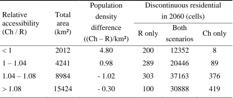
areas far from stations. Obviously, the ‘choice’ scenario is, by definition, much more
realistic than the theoretical ‘train only’ scenario, yet its results do not differ much from
those of the ‘road-based’ scenario (Table 5). This is clearly caused by the values of the
modal weights w in the ‘choice’ scenario, but we chose these values because it is
reasonable that the road network plays the most important role in allocating new land
uses, especially in the many suburban villages and ribbon developments of Belgium. In
comparison with the ‘road-based’ scenario there is a slightly higher population growth
near the most important stations. On the contrary, residential land-use growth is slightly
greater near the edge of these cities in less accessible cells of this scenario. This may seem
contra-intuitive but it is caused by the attraction effects of the model since there is no
space for urban growth very close to major stations.
[Table 3 about here]
[Table 4 about here]
[Table 5 about here]
Although the variable grid provides a good computational framework for activity
predictions in large study areas, network distance calculations can be further improved.
of NG cells, of which one may represent the centroid of a larger variable grid supercell.
The latter might not be representative of the location of the activities within the supercell.
Hence, the logical next step is to represent each supercell by a centre that reflects the
actual distribution of activity within the supercell. Initial tests of this approach are
generally positive, but more work is necessary to define the best way of implementing it.
Secondly, the access and egress legs in the multimodal computations can be made more
realistic, since in home-to-work travel there is often a very short leg at the work end of
the displacement (Thys and Andries, 2011). Because of the symmetry of the variable grid,
such an asymmetric approach has not yet been implemented.
Extra details could also be included in an improved transport-based model, such
as different modal weights w for different regions of the study area, or transport networks
evolving over time. The functionality to introduce changes to the network at specified
time steps during a simulation is already implemented, but has not been used due to a lack
of data. Since Belgium already has a dense network, there are likely to be few additions
to the network, but a growing population and increased congestion could reduce travel
speeds in the future, and road characteristics could change. Congestion scenarios of
transport models can therefore provide useful input for the model. It would be an
interesting exercise to couple our activity based CA model directly to a transport model
in order to get simultaneous predictions of activities, land uses and transport for the future.
On the other hand, we fear that a direct coupling would increase the computation time
drastically.
Finally, in a more complete and general sensitivity analysis it would be interesting
to examine how parameters, rules and functions of the activity based CA could be
adapted, added or removed to improve the model. For instance, the accessibility
influence in the network-based implementation, and so it might be redundant.
Additionally, it would be interesting to use a generalized cost measure of distance. Such
a measure would enable the model to be used to investigate the effects of a subsidised,
and hence cheaper, public transport in comparison with congestion pricing schemes for
the road network.
7. Conclusion
The activity-based CA model of White et al. (2012) was a big step forward in comparison
with earlier CA models, since every cell is modelled as a truly multifunctional
environment where people live and work. Future versions of this model could even
include agricultural yield or natural activities as a complement to the current,
predominantly urban activities. In this study, we developed an activity-based CA model
with travel time-based interaction rules for long-distance interactions, and simple
Euclidean distance-based rules for the local vicinity interactions. The network-based rule
sets for the model are clearly more realistic and provide the possibility to test different
transport scenarios. The impacts of road congestion and public transport usage on
land-use and activity futures can be evaluated with the proposed approach, and possibly new
spatial indicators could be derived to clearly display these impacts.
Nevertheless, the new version of the model still has some shortcomings. The
variable grid could be adapted by defining activity centres as the representative locations
of large variable grid cells, of which some can only be reached by road and others both
by road and public transport. Furthermore, more critical assessment, calibration and
sensitivity analysis are needed to confirm that all its current components are useful and
necessary, and to update parameters and rule sets.
The application to Belgium is interesting since the country could benefit from
continue this work with a historical calibration exercise to validate and improve the
model. Enhanced model versions could be used to promote sustainable land-use scenarios
and provide the relevant decision-makers with better insights into the coupled problems
of growing congestion and urban sprawl.
Acknowledgements
This work is supported by a PhD scholarship financed by the Flemish Institute for Technological
Research (VITO), Environmental Modelling Unit, Mol, Belgium.
References
Aljoufie, M., et al., 2013. A cellular automata-based land use and transport interaction
model applied to Jeddah, Saudi Arabia. Landscape and Urban Planning, 112, 89–99.
Almeida, C.M., et al., 2008. Using neural networks and cellular automata for modelling
intra-urban land-use dynamics. International Journal of Geographical Information
Science, 22, 943–963.
Andersson, C., Rasmussen, S., and White, R., 2002a. Urban settlement transitions.
Environment and Planning B: Planning and Design, 29, 841–865.
Andersson, C., et al., 2002b. Urban growth simulation from first principles. Physical
Review E, 66, 1–9.
Antrop, M., 2000. Changing patterns in the urbanized countryside of Western Europe.
Landscape Ecology, 15, 257–270.
Baetens, J.M., De Loof, K., and De Baets, B., 2013. Influence of the topology of a cellular
automaton on its dynamical properties. Communications in Nonlinear Science and
Numerical Simulation, 18, 651–668.
Barredo, J.I., et al., 2003. Modelling dynamic spatial processes: simulation of urban
future scenarios through cellular automata. Landscape and Urban Planning, 64,
Batty, M., 2005. Cities and Complexity: Understanding Cities with Cellular Automata,
Agent-Based Models, and Fractals. Cambridge, MA: The MIT Press.
Berens, W., 1988. The suitability of the weighted lp-norm in estimating actual road
distances. European Journal of Operational Research, 34, 39-43.
Blečić, I., Cecchini, A, and Trunfio, G.A., 2011. Modelling proximal space in urban cellular automata. In: B. Murgante, et al., eds. Proceedings of the 11th International Conference on Computational Science and Its Applications (ICCSA 2011), Part I, 20–
23 June 2011, Santander, Spain, 477–491.
Boussauw, K., Derudder, B., and Witlox, F., 2011. Measuring spatial separation
processes through the minimum commute: the case of Flanders. European Journal of
Transport and Infrastructure Research, 11, 42–60.
Boussauw, K., Neutens, T., and Witlox, F., 2012. Relationship between spatial proximity
and travel-to-work distance: the effect of the compact city. Regional Studies, 46, 687–
706.
Brimberg, J., Walker, J.H., and Love, R.F., 2007. Estimation of travel distances with the
weighted lp norm: Some empirical results. Journal of Transport Geography, 15, 62–72.
Bura, S., et al., 1996. Multiagent systems and the dynamics of a settlement system.
Geographical Analysis, 28, 161–178.
Camagni, R., Gibelli, M.C., and Rigamonti, P., 2002. Urban mobility and urban form: the
social and environmental costs of different patterns of urban expansion. Ecological
Economics, 40, 199–216.
Chang, J.S., 2006. Models of the relationship between transport and land-use: a review.
Transport Reviews, 26, 325–350.
De Decker, P., 2011. Understanding housing sprawl: the case of Flanders, Belgium.
Environment and Planning A, 43, 1634–1654.
de Kok, J.-L., et al., 2012. Spatial dynamic visualization of long-term scenarios for
al., eds. Proceedings of the 6th International Congress on Environmental Modelling and Software, 1–5 July 2012, Leipzig, Germany, 1984–1991.
Dijkstra, E.W., 1959. A note on two problems in connexion with graphs. Numerische
Mathematik, 1, 269–271.
Echenique, M., 2004. Econometric models of land use and transportation. In: D.A.
Hensher, et al., eds. Handbook of Transport Geography and Spatial Systems. Kidlington,
UK: Pergamon/Elsevier Science: 185–202.
Engelen, G., et al., 1995. Using cellular automata for integrated modelling of
socio-environmental systems. Environmental Monitoring and Assessment, 34, 203–214.
Engelen, G., et al., 2007. The MOLAND modelling framework for urban and regional
land use dynamics. In: E. Koomen, et al., eds. Modelling Land-Use Change: Progress
and Applications. Springer, 297–320.
Fuglsang, M., Hansen, H.S., and Münier, B., 2011. Accessibility Analysis and Modelling
in Public Transport Networks – A Raster Based Approach. In: B. Murgante, et al., eds.
Proceedings of the 11th International Conference on Computational Science and Its Applications (ICCSA 2011), Part I, 20–23 June 2011, Santander, Spain, 207–224.
Fuglsang, M., Münier, B., and Hansen, H.S., 2013. Modelling land-use effects of future
urbanization using cellular automata: An Eastern Danish case. Environmental Modelling
& Software, 50, 1-11.
Geertman, S. and Stillwell, J., eds., 2009. Planning Support Systems Best Practice and
New Methods. Dordrecht: Springer.
Gilbert, N., 2008. Agent-Based Models. In: Quantitative Applications in the Social
Sciences, 153. London: Sage.
Giuliano, G. and Dargay, J., 2006. Car ownership, travel and land use: a comparison of
the US and Great Britain. Transportation Research Part A, 40, 106–124.
Haase, D. and Schwarz, N., 2009. Simulation models on human-nature interactions in
urban landscapes: a review including spatial economics, system dynamics, cellular
Available from http://landscaperesearch.livingreviews.org/Articles/lrlr-2009-2/
[Accessed 18 February 2014].
Hagen-Zanker, A., 2012. A comparison of three urban models of land use, transport and
activity. In: N.N. Pinto, J. Dourado, and A. Natálio, eds. Proceedings of the International
Symposium on Cellular Automata Modeling for Urban and Spatial Systems (CAMUSS),
8–10 November 2012, Porto, Portugal, 337–338.
Hagen-Zanker, A. and Jin, Y., 2012. A new method of adaptive zoning for spatial
interaction models. Geographical Analysis, 44, 281–301.
Hagen-Zanker, A. and Jin, Y., 2013. Adaptive zoning for transport mode choice
modelling. Transactions in GIS, 17, 706–723.
Handy, S., Cao, X., and Mokhtarian, P., 2005. Correlation or causality between the built
environment and travel behavior? Evidence from Northern California. Transportation
Research Part D: Transport and Environment, 10, 427–444.
Hansen, H.S., 2009. Analysing the role of accessibility in contemporary urban
development. In: O. Gervasi, et al., eds. Proceedings of the International Conference on
Computational Science and Its Applications – ICCSA 2009, Part I, 29 June – 2 July 2009, Seoul, Korea, 385–396.
Hansen, H.S., 2010. Modelling the future coastal zone urban development as implied by
the IPCC SRES and assessing the impact from sea level rise. Landscape and Urban
Planning, 98, 141–149.
Hoornaert, S., et al., 2014. Verkeersindicatoren hoofdwegennet Vlaanderen 2013.
Antwerp: Flemish Traffic Study Centre (Vlaams Verkeerscentrum). Available from
http://www.verkeerscentrum.be/pdf/rapport-verkeersindicatoren-2013-v1.pdf [Accessed
8 July 2014].
Iacono, M., Levinson, D., and El-Geneidy, A., 2008. Models of transportation and land
use change: a guide to the territory. Journal of Planning Literature, 22, 323–340.
Lambin, E.F. and Geist, H., eds., 2006. Land-Use and Land-Cover Change. Local
Lauf, S., et al., 2012. Uncovering land-use dynamics driven by human decision-making – A combined model approach using cellular automata and system dynamics. Environmental Modelling & Software, 27–28, 71–82.
Matthews, R.B., et al., 2007. Agent-based land-use models: a review of applications.
Landscape Ecology, 22, 1447–1459.
Næss, P., 2010. Residential location, travel, and energy use in the Hangzhou Metropolitan
Area. Journal of Transport and Land Use, 3, 27–59.
Newman, P. and Kenworthy, J., 1989. Cities and Automobile Dependence. A Sourcebook.
Aldershot: Gower.
Parker, D.C., et al., 2003. Multi-Agent systems for the simulation of land-use and
land-cover change: A review. Annals of the Association of American Geographers, 93,
314–337.
Parry, H.R. and Bithell, M., 2012. Large scale agent-based modelling: a review and
guidelines for model scaling. In: A.J. Heppenstall, et al., eds. Agent-based Models of
Geographical Systems. Springer Netherlands, 271–308.
Poelmans, L. and Van Rompaey, A., 2009. Detecting and modelling spatial patterns of
urban sprawl in highly fragmented areas: A case study in the Flanders-Brussels region.
Landscape and Urban Planning, 93, 10–19.
Poelmans, L. and Van Rompaey, A., 2010. Complexity and performance of urban
expansion models. Computers, Environment, and Urban Systems, 34, 17–27.
Ravetz, J., Fertner, C., and Nielsen, T.S., 2013. The dynamics of peri-urbanization. In:
K. Nilsson, et al., eds. Peri-urban futures: Scenarios and models for land use change in
Europe. Berlin/Heidelberg: Springer-Verlag, 13–44. Santé, I., et al., 2010. Cellular
automata models for the simulation of real-world urban processes: A review and analysis.
Landscape and Urban Planning, 96, 108–122.
Schwanen, T. and Mokhtarian, P.L., 2005. What affects commute mode choice:
neighborhood physical structure or preferences toward neighborhoods? Journal of
Sohn, J., 2005. Are commuting patterns a good indicator of urban spatial structure?
Journal of Transport Geography, 13, 306–317.
Stanilov, K. and Batty, M., 2011. Exploring the historical determinants of urban growth
patterns through cellular automata. Transactions in GIS, 15, 253–271.
Thys, B. and Andries, P., 2011. Diagnostiek Woon-Werkverkeer van 30 juni 2011.
Brussels: Belgian Federal Department of Mobility and Transport.
United Nations, 2013. World Population Prospects: The 2012 Revision, Key Findings
and Advance Tables. Working Paper No. ESA/P/WP.227. New York: United Nations,
Department of Economic and Social Affairs, Population Division. Available from
http://esa.un.org/wpp/Documentation/pdf/WPP2012_%20KEY%20FINDINGS.pdf
van de Coevering, P. and Schwanen, T., 2006. Re-evaluating the impact of urban form
on travel patterns in Europe and North-America. Transport Policy, 13, 229–239.
Vandenbulcke, G., Steenberghen, T., and Thomas, I., 2009. Mapping accessibility in
Belgium: a tool for land-use and transport planning? Journal of Transport Geography,
17, 39–53.
Van Steertegem, M., et al., eds., 2009. Milieuverkenning 2030. Milieurapport
Vlaanderen, MIRA 2009. Erembodegem: Vlaamse Milieumaatschappij. Available from
http://www.milieurapport.be/nl/publicaties/toekomstverkenningen/milieuverkenning-2030/
van Vliet, J., White, R., and Dragicevic, S., 2009. Modeling urban growth using a variable
grid cellular automaton. Computers, Environment and Urban Systems, 33,
35–43.
van Vliet, J., et al., 2012. An activity based cellular automaton model to simulate land
use dynamics. Environment and Planning B: Planning and Design, 39, 198–212.
Waddell, P., 2002. UrbanSim: Modeling Urban Development for Land Use,
Transportation and Environmental Planning. Journal of the American Planning
Wegener, M., 2004. Overview of land-use transport models. In: D.A. Hensher, et al., eds.
Handbook of Transport Geography and Spatial Systems. Kidlington, UK:
Pergamon/Elsevier Science, 127–146.
White, R., 2006. Modelling multi-scale processes in a cellular automata framework. In:
J. Portugali, ed., Complex Artificial Environments. Berlin/Heidelberg: Springer-Verlag,
165–178.
White, R. and Engelen, G., 2000. High resolution integrated modelling of the spatial
dynamics of urban and regional systems. Computers, Environment, and Urban Systems,
24, 383–400.
White, R., Engelen, G., and Uljee, I., 1997. The use of constrained cellular automata for
high-resolution modelling of urban land-use dynamics. Environment and Planning B:
Planning and Design, 24, 323–343.
White, R., Shahumyan, H., and Uljee, I., 2011. Activity based variable grid cellular
automata for urban and regional modelling. In: D. Marceau and I. Benenson, eds.
Advanced Geosimulation Models. Hilversum, The Netherlands: Bentham, 14–29.
White, R., Uljee, I., and Engelen, G., 2012. Integrated modelling of population,
employment and land-use change with a multiple activity-based variable grid cellular
Table 1. Average modelling speeds for road segments in km/h.
Link type Legal max. speed
(reality)
Average speed
(model)
Motorway 120 100
Express road, urban motorway 90-100 85
Major road 90 70
Secondary road 70 55
Local road 50 40
Urban low speed zone 30 30
‘Euclidean speed’ - 5
Table 2. Land-use and activity growth scenarios, and parameter values of the
application to Belgium that were copied from White et al. (2012).
Active land use or activity Value in 2000 Value in 2060
Discontinuous urban fabric (cells) 56,051 101,741
Continuous urban fabric (cells) 527 570
Industrial or commercial units (cells) 5540 6000
Population 10,251,249 12,662,761
‘Urban’ employment 855,822 891,061
[image:35.595.71.522.385.530.2]Table 3. Comparison in 2060, in terms of discontinuous residential land use and
population, between the ‘road-based’ scenario (‘R’) and the ‘congestion’ scenario (‘C’).
The classes are defined by relative accessibility index values (division of ‘congestion’
and ‘road-based’ index values).
Relative accessibility (C / R)
Total area (km²) Population density difference
((C – R)/km²)
Discontinuous residential
in 2060 (cells)
R only Both
scenarios C only
< 0.97 9493 3.11 192 12911 222
0.97 – 1 6731 9.80 89 19349 516
1 – 1.15 8746 8.03 572 36577 1276
> 1.15 5692 - 29.11 1806 30245 645
Table 4. Comparison in 2060, in terms of discontinuous residential land use and
population, between the ‘road-based’ scenario (‘R’) and the ‘train only’ scenario (‘T’).
The classes are defined by relative accessibility index values (division of ‘train only’
and ‘road-based’ index values).
Relative accessibility (T / R)
Total area (km²) Population density difference
((T – R)/km²)
Discontinuous residential
in 2060 (cells)
R only Both
scenarios T only
< 1 597 160.62 5 4140 384
1 – 2 5774 53.96 551 24242 2370
2 – 3 14408 - 11.13 4325 41484 5163
[image:36.595.124.476.475.635.2]Table 5. Comparison in 2060, in terms of discontinuous residential land use and
population, between the ‘road-based’scenario (‘R’) and the ‘choice’ scenario (‘Ch’).
The classes are defined by relative accessibility index values (division of ‘choice’ and ‘road-based’ index values).
Relative accessibility (Ch / R)
Total area (km²)
Population
density
difference
((Ch – R)/km²)
Discontinuous residential
in 2060 (cells)
R only Both
scenarios Ch only
< 1 2012 4.80 200 12352 8
1 – 1.04 4241 0.98 289 20446 89
1.04 – 1.08 8984 - 1.02 303 37163 376
Figure 1. Structure of the variable grid.
Figure 2. Example of a neighbourhood influence function for the variable grid activity
[image:38.595.113.475.481.676.2]