Autonomous crowds tracking with box particle filtering and convolution particle filtering

(1)

Contents lists available atScienceDirect

Automatica

journal homepage:www.elsevier.com/locate/automatica

Autonomous crowds tracking with box particle filtering and

convolution particle filtering

✩

Allan De Freitas

a

,

Lyudmila Mihaylova

a

,

Amadou Gning

b

,

Donka Angelova

c

,

Visakan Kadirkamanathan

a

a_{Department of Automatic Control and Systems Engineering, University of Sheffield, United Kingdom} b_{Department of Computer Science, University of Hull, United Kingdom}

c_{Institute of Information and Communication Technologies, Bulgarian Academy of Sciences, Bulgaria}

a r t i c l e i n f o

Article history:

Received 23 January 2015 Received in revised form 11 January 2016

Accepted 26 February 2016

Keywords: Box particle filter Convolution particle filter Crowd tracking

a b s t r a c t

Autonomous systems such as Unmanned Aerial Vehicles (UAVs) need to be able to recognise and track crowds of people, e.g. for rescuing and surveillance purposes. Large groups generate multiple measurements with uncertain origin. Additionally, often the sensor noise characteristics are unknown but measurements are bounded within certain intervals. In this work we propose two solutions to the crowds tracking problem— with a box particle filtering approach and with a convolution particle filtering approach. The developed filters can cope with the measurement origin uncertainty in an elegant way, i.e. resolve the data association problem. For the box particle filter (PF) we derive a theoretical expression of the generalised likelihood function in the presence of clutter. An adaptive convolution particle filter (CPF) is also developed and the performance of the two filters is compared with the standard sequential importance resampling (SIR) PF. The pros and cons of the two filters are illustrated over a realistic scenario (representing a crowd motion in a stadium) for a large crowd of pedestrians. Accurate estimation results are achieved.

1. Introduction

Tracking a large number of objects requires scalable algorithms that are able to deal with large volumes of data characterised by the presence of clutter. Although groups are made up of many indi-vidual entities, they typically maintain certain patterns of motion, such as in the case of crowds of pedestrians (Ali & Dailey, 2009). When the number of objects in the group is huge, e.g. hundreds and thousands, it is impractical (and impossible) to track them all indi-vidually. Instead of tracking each separate component, the group can be considered as one whole entity. Large group techniques identify and track concentrations, typically the kinematic states of the group and its extent parameters (Koch, 2008).

✩ _{The material in this paper was presented at the 15th International conference}

in Information Fusion, July 9–12, 2012, Singapore and the 17th International Conference in Information Fusion, July 7–10, 2014, Salamanca, Spain. This paper was recommended for publication in revised form by Associate Editor Huijun Gao under the direction of Editor Ian R. Petersen.

E-mail addresses:[email protected](A. De Freitas),

[email protected](L. Mihaylova),[email protected](A. Gning), [email protected](D. Angelova),[email protected](V. Kadirkamanathan).

Recent results for the modelling, simulating and visual analysis of crowds are presented inAli, Nishino, Manocha, and Shah(2014) from the point of view of computer vision, transportation systems and surveillance. The social force model (Ali et al.,2014;Helbing & Molnár, 1995;Mazzon & Cavallaro, 2013) has been used to model behaviour of pedestrians, including evacuation of people through bottlenecks. The social force model has also been combined with some filtering techniques for multiple-target tracking inPellegrini, Ess, Schindler, and Van Gool(2009).

There is a wealth of approaches that are developed to track kinematic states of large crowds (e.g. the centre of the crowds) and their size (extent parameters). A recent survey (Mihaylova et al., 2014) presents key trends in the area. Although, the problem of tracking large groups has received attention in the literature, it is far from being resolved due to the various challenges that are present. Some of these challenges involve difficulties in modelling the interactions between the entities of the crowd, data association and dynamic shape changes of the crowd. Some of the approaches that have been proposed include mixtures of Gaussian components (Carmi, Septier, & Godsill, 2012) and a wealth of Random finite sets (RFS) methods, e.g.,Grandström(2012),Granström, Lundquist, and Orguner(2011),Mahler (2007,2009,2013)andMahler and Zajic (2002).

http://dx.doi.org/10.1016/j.automatica.2016.03.009

(2)

This work proposes two novel solutions to the crowd tracking problem based on the recently developed box particle filter (PF) (Gning, Ristic, Mihaylova, & Abdallah, 2013) and convolution particle filter (CPF) (Angelova, Mihaylova, Petrov, & Gning, 2013; Campillo & Rossi, 2009;Rossi & Vila, 2006) frameworks.

The box PF (Abdallah, Gning, & Bonnifait, 2008; Gning, Mihaylova, Abdallah, & Ristic, 2012;Gning et al.,2013) relies on the concept of a box particle, which occupies a small and controllable rectangular region having a non-zero volume in the state space. The box PF affords to resolve the data association problems arising from the multiple measurements originating from the crowd. This is a common case when a UAV is flying over a region and collects data, seeing the area from above.

This paper has several novel contributions when compared with our previous works such asPetrov, Gning, Mihaylova, and Angelova (2012),Petrov, Ulmke et al.(2012) andPetrov, Mihaylova, de Fre-itas, and Gning(2014). These novelties include: (i) a generalised likelihood function for the box PF is derived when the state vec-tor consists of kinematic states and extent parameters; (ii) the likelihood of the Box PF is calculated based on optimisation, by solving a constraint satisfaction problem (CSP) with multiple mea-surements; (iii) the online estimation of the crowd and clutter measurement rates; (iv) an adaptive CPF is proposed. The devel-oped CPF is able to deal with multiple measurements, including a high level of clutter. It is able to resolve the data association prob-lem without the crowd and clutter measurement rates. The adap-tive CPF can estimate both dynamic kinematic states and dynamic parameters which is a different solution from the CPF based ap-proach for static parameters presented inAngelova et al.(2013), Campillo and Rossi(2009) andRossi and Vila(2006).

Both filters have very appealing properties in solving nonlinear estimation problems. Both filters operate in the condition of uncertain and imperfect observations: fluctuating number of sensor reports.

The performance of the box PF and CPF is evaluated for two different cases. Firstly, in a fully matched case where the models used by the filter directly match that used by the simulator, and secondly, in an unmatched scenario of a realistic crowd moving through a bottleneck. Both filters are compared with the standard sequential importance resampling PF (SIR PF) (Doucet, De Freitas, & Gordon, 2001) in terms of filter accuracy and computational complexity.

A main advantage of the box PF consists in its robustness to measurement characteristics and its ability to be implemented efficiently in a distributed way. The CPF is based on the principles of kernel based learning and can deal with problems where the likelihood is not available in an analytical form or it is difficult to calculate.

The rest of this paper is organised in the following way. Section2describes the state space modelling of a crowd. Section3 is a brief overview of inference in a Bayesian framework. Section4 presents the adaptation of the box PF for group object tracking. Section5introduces the CPF for crowd tracking, which is followed by a performance evaluation of the presented approaches in Section6. Finally, conclusions are presented in Section7.

2. State space modelling of a crowd

The characteristics of the crowd and scene that are required to be inferred at each time stepk

,

k

=

1

,

2

, . . . ,

K, are represented by an augmented state vector:

ζ

k

=



λ

T

k

,

X T k

,

2

T k



T

,

(1)

whereXkis the kinematic vector of the centre of the crowd, and

2kis the parameter vector which characterises the crowd extent.

Multiple measurements are received from the crowd and from clutter at each time step, thus the state vector includes

λ

_kwhich is the measurement rate vector. The notation

(

· )

T_{is the transpose}

operator. In this paper we consider the two-dimensional case, where the kinematic vector consists of the position coordinates and the velocity of the centre of the crowd and the extent of the crowd is represented by a rectangle. The resulting kinematic vector has the following form:

Xk

=

(

xk

,

x

˙

k

,

yk

,

y

˙

k

)

T (2)

and the parameter vector is given by:

2k

=

(

ak

,

bk

)

T (3)

whereakandbkrepresent the lengths of the sides of the rectangle

in the xand ydimensions, respectively. The measurement rate vector is represented by:

λ

k

=

(λ

T,k

, λ

C,k

)

T

,

(4)

where

λ

T,kand

λ

C,krepresent the crowd and clutter measurement

rates, respectively.

2.1. Crowd dynamics model

The motion of the centre of the crowd is modelled by a correlated velocity model. The correlated velocity model is related to the Singer model (Singer, 1970) and jerk model (Mehrotra & Mahapatra, 1997) with the difference being that the velocity component is correlated in time and that the second and other higher order derivatives of position are negligible. The evolution model for the kinematic state of the target is represented mathematically by

Xk

=

AXk−1

+

η

k

,

(5)

where

η

_k represents the system dynamics noise. The state transition matrix is given by

A

=





1 1

α



1

−

e−αTs



0 e−αTs





⊗

I2 (6)

where Ts is the sampling interval,

⊗

denotes the Kronecker

product,I2denotes the 2

×

2 identity matrix, and

α

is the reciprocal

of the velocity correlation time constant. The covariance of the system dynamics noise

η

_kcan be modelled as

Q

=

2

ασ

_v2



q11 q12 q12 q22



⊗

I2

,

(7)

where

σ

_v2is the variance of the velocity of the crowd centroid for a single dimension and

q11

=

1 2

α

3



4e−αTs

₋

₃

₋

_e−2αTs

₊

₂

α

_T

s



,

q12

=

1 2

α

2



e−2αTs

₊

₁

₋

₂_e−αTs



,

q22

=

1

2

α



1

−

e−2αTs



.

(8)

The evolution for the crowd extent is assumed to be a random walk model, described by

2k

=

2k−1

+

η

p,k

,

(9)

(3)

2.2. Observation model

In this paper we consider the scenario where the measurements originate from within a confined area. However, other scenarios, such as the case where the measurements only come from the border of the crowd, have a similar solution.

The total number of measurementsMk, obtained at each time

step from the sensor consists of theMT,k number of

measure-ments, originating from the crowd andMC,kclutter measurements,

i.e.Mk

=

MT,k

+

MC,k. The number of measurementsMT,k

origi-nating from the crowd is considered as a Poisson-distributed ran-dom variable with mean value of the crowd rate,

λ

T,k, i.e.,MT,k

∼

Poisson

(λ

T,k

)

. Similarly, the number of clutter measurements is

MC,k

∼

Poisson

(λ

C,k

)

. TheMT,kmeasurements originating from the

crowd are uniformly located in the area represented by the crowd. TheMC,kclutter measurements are uniformly located in the region

about the crowd.

Typically in point target tracking, an observation model which directly relates the states to the measurements is available, in the form given by:

zk

=

h

(

ζ

k

)

+

ξ

k

,

(10)

where

ξ

_k represents the observation noise. However, since the crowd is an extended target,1there is no direct observation model. The observations can be indirectly related to the states through the sensor characteristics and the target model.

The sensor characteristics describe the relationship between the measurement pointm

,

m

=

1

, . . . ,

Mkand the measurement

source in a Cartesian coordinate system and is of the form:

z_km

= ˜

h

(

xm_k

)

+

ξ

_k

,

(11) where _h

˜

₍

· )

is the measurement function andxm

k

=

(

xmk

,

ymk

)

T

denotes the Cartesian coordinates of the measurement source in a two dimensional space. In this paper we consider the following model:

z_km

=

Hxm_k

+

ξ

_k

,

(12)

whereH

=

I2, and the measurement noise

ξ

k

=

(ξ

1,k

, ξ

2,k

)

T,

is assumed (but not restricted) to be Gaussian, with a known covariance matrix R

=

diag

(σ

2

1

, σ

22

)

. The vector of interval

measurements is

[

z_km

] =

(

[z

₁m_,_k

]

,

[z

m₂_,_k

]

)

T, where

[z

₁m_,_k

]

and

[z

₂m_,_k

]

are the intervals of themth measurement point. One way to describe these components is by representing the noise terms in Eq.(11)as intervals:

[

ξ

_k

] = [−

3

σ

,

+

3

σ

]

.

(13)

At each time stepk, theMkinterval measurements are combined

into an interval matrix

[

Zk

] = {[

zk1

]

, . . . ,

[

zkm

]} ∈

Rn

z×Mk_.

Each measurement originates from either random clutter or the crowd but its origin is unknown. The target model describes the relationship between the states and the measurement sources for the MT,k measurements that originate from the crowd. As

previously described, the measurement sources are uniformly distributed across the region which exhibits measurements, and this region is represented by the states through the following probability density:

p

(

xm_k

|

xk

)

=

Uq(xk)

(

x

m

k

),

(14)

whereU[x]

(

· )

denotes the multivariate uniform probability density

function (pdf) with the interval

[

x

]

as support. The support of the uniform distribution describes two independent regions which

1 Anextended targetcannot be considered as a point, but instead it has a physical extent characterising its size and volume.

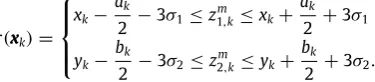
cover the area of the rectangle used to approximate the extent of the crowd:

q

(

xk

)

=











xk

−

ak

2

≤

x

m k

≤

xk

+

ak

2

,

yk

−

bk

2

≤

y

m k

≤

yk

+

bk

2

.

(15)

3. Inference in a Bayesian framework

Classic Bayesian inference relies on computing the posterior distribution from a prior distribution and measurements. The posterior distribution can be updated sequentially based on a prediction step, followed by an update step. The following equation describes the prediction:

p

(

ζ

_k

|

Z1:k−1

)

=



Rnζ

p

(

ζ

_k

|

ζ

_k₋₁

)

p

(

ζ

_k₋₁

|

Z1:k−1

)

d

ζ

k−1

.

(16)

The measurement update is described by the following equation:

p

(

ζ

_k

|

Z1:k

)

=

p

(

Zk

|

ζ

k

)

p

(

ζ

k

|

Z1:k−1

)

p

(

Zk

|

Z1:k−1

)

.

(17)

The recursive relationship of Eqs.(16)and(17)forms the optimal Bayesian solution. Utilising these equations for Bayesian filtering is generally not possible since an analytical solution rarely exists. A solution for when the state space model is linear and perturbed by Gaussian noise is referred to as the Kalman filter (Bar-Shalom, Li, & Kirubarajan, 2001). Several techniques have been used in the more general case consisting of non-linearities and non-Gaussianity in the state space model, such as the extended Kalman filter ( Bar-Shalom et al., 2001), unscented Kalman filter (Wan & Van Der Merwe, 2000) and particle filter based techniques (Cappe, Godsill, & Moulines, 2007) to name a few.

For further notational convenience, the marginal state is defined as follows:

xk

=



X_kT

,

2T_k



T

.

(18)

In this application the posterior distribution can be further factored into the following form:

p

(

ζ

_k

|

Z1:k

)

=

p

(

xk

|

Z1:k

,

λ

k

)

p

(λ

T,k

|

Z1:k

)

p

(λ

C,k

|

Z1:k

).

(19)

This factorisation implicitly states that the crowd and clutter measurement rates are independent of the kinematics and extent of the crowd. This is true for the clutter measurement rate but not necessarily valid for the crowd measurement rate. However, the variance of the prior distribution for the crowd rate is sufficient to represent the variation of the number of measurements over time. It has been shown that a closed form recursive Bayesian so-lution exists for the estimation of the mean of a Poisson distri-bution, based on using the conjugate prior Gamma distribution (Granström & Orguner, 2012). The crowd and clutter measurement rates are estimated based on this concept,2_{and the focus of this} paper thus lies on the calculation of the marginal posterior distri-bution for the states representing the kinematics and extent of the crowd,p

(

xk

|

Z1:k

,

λ

k

)

, using the novel box particle filter and

convo-lution particle filter algorithms.

4. The box particle filter for crowd tracking

This section begins with a review of the box PF in point target tracking without clutter, thus, the following subsection does not consider the extent of the target, i.e.xk

=

Xk.

(4)

4.1. The classic box particle filter

The concept of abox particleis introduced where a box particle represents a small region with controllable size (or volume). The box PF approximates the posterior state pdf with a mixture of uniform pdfs (Gning, Mihaylova, & Abdallah, 2010; Gning, Mihaylova et al.,2012), i.e.

p

(

xk−1

|

z1:k−1

)

≈

N



p=1

w

(p)

k−1U[x_k(p₋)₁]

(

xk−1

).

(20)

For the box PF, the time update can be written as:

p

(

xk

|

z1:k−1

)

≈



Rnx

p

(

xk

|

xk−1

)

N



p=1

w

(p)

k−1U[x(_kp₋)₁]

(

xk−1

)

dxk−1

=

N



p=1

w

(p) k−1



[x(_kp₋)₁]

p

(

xk

|

xk−1

)

U_[_x(p) k−1]

(

xk−1

)

dxk−1

.

(21)

For any transition functionf, we can obtain an inclusion function

[f

]

wheref

(

[

x

]

)

⊆ [f

]

(

[

x

]

)

. For the inclusion function, with

∀

p

=

1

, . . . ,

N, ifxk−1

∈ [

x(kp−1)

]

we havexk

∈ [f

]

(

[

xk(p−1)

]

)

+ [

η

k

]

. Thus, for

allp

=

1

, . . . ,

Nwe can write

p

(

xk

|

xk−1

)

U_[_x(p) k−1]

(

xk−1

)

=

0

,

∀

xk

̸∈ [f

]

(

[

x(kp−1)

]

)

+ [

η

k

]

.

(22)

Using interval analysis techniques, the support function3_{for the} pdf terms in (21) can be approximated by

[f

]

(

[

x(_kp₋₁)

]

)

+ [

η

_k

]

. In the Box PF algorithm each pdf term in(21)is approximated by one uniform pdf component having as support the interval

[f

]

(

[

x_k(p₋₁)

]

,

[

η

_k

]

)

, i.e.,



[x(_kp₋)₁]

p

(

xk

|

xk−1

)

U_[_x(p)

k−1]

(

xk−1

)

dxk−1

≈

U_[_f_]₍_[_x(p)

k−1])+[ηk]

(

xk

).

(23)

Combining(21)and(23)gives

p

(

xk

|

z1:k−1

)

≈

N



p=1

w

(p)

k−1U[f]([x_k(p₋)₁])+[ηk]

(

xk

)

=

N



p=1

w

(p)

k−1U[x_k(p_|_k)₋₁]

(

xk

).

(24)

Approximating each pdf term using one uniform pdf component may not be accurate enough. However, as for the PF, it is sufficient to approximate the first moments of the pdf. If a more accurate representation is required then each term can be approximated as a mixture of uniform pdfs as shown inGning, Mihaylova et al. (2012).

Under the assumption that at time instantk, the time update pdfp

(

xk

|

z1:k−1

)

can be represented by a mixture ofNuniform pdfs

with interval supports

[

x(_k_|p_k)₋₁

]

and weights

w

p_k₋₁, the measurement update step can be performed. A probabilistic modelp_ξ for the measurement noise

ξ

_kis also available. It is assumed in general thatp_ξcan be expressed by using a mixture of uniform pdfs. For simplicity and without loss of generality,p_ξis considered here to be a single uniform pdf, such that the box measurement

[

zk

]

contains

all realisations of(10). Then we have:p

(

zk

|

xk

)

=

U[zk]

(

h

(

xk

))

and

according to Eq.(17), the measurement update can be expressed

3 The support of a function is the set of points where the function is not zero-valued or, in the case of functions defined on a topological space, the closure of that set.

with the equation:

p

(

xk

|

z1:k

)

=

1

α

k

p

(

zk

|

xk

)

p

(

xk

|

z1:k−1

)

=

1

α

k

U[zk]

(

h

(

xk

))

N



p=1

w

(p)

k−1U[x_k(p_|_k)₋₁]

(

xk

)

=

1

α

k N



p=1

w

(p)

k−1U[zk]

(

h

(

xk

))

U[x(_kp_|_k)₋₁]

(

xk

),

(25)

where

α

k denotes the normalising constant. Each of the terms

U[zk]

(

h

(

xk

))

U[x_k(p_|_k)₋₁]

(

xk

)

is also a constant function with a support

being the following regionSp

⊂

Rnx, where

Sp

=



xk

∈ [

x(kp|k)−1

] |

h

(

xk

)

∈ [

zk

]



.

(26)

Eq.(26)represents a constraint and from its expression we can deduce that predicted supports

[

x(_kp_|_k)₋₁

]

, from the time update pdf

p

(

xk

|

z1:k−1

)

approximation, have to be contracted with respect to

the measurement

[

zk

]

. These contraction steps result in the new

box particles denoted

[

x(_kp)

]

, which approximate the posterior pdf

p

(

xk

|

z1:k

)

at timek. Following the definition of the setsSpin(26),

we can write

U[zk]

(

h

(

xk

))

U[x(_kp_|_k)₋₁]

(

xk

)

≃

U[zk]

(

h

(

xk

))

1

|[

x(_kp_|_k)₋₁

]|

∥S

p

∥U

Sp

(

xk

),

(27)

where

| · |

denotes the interval length (respectively the box volume in the multidimensional case). By combining Eqs.(25)and(27), and keeping in mind that

[

x(_kp)

] = [S

p

]

(i.e. by definition

[

x(kp)

]

is the

smallest box containingSp),

p

(

xk

|

z1:k

)

=

1

α

k

N



p=1

w

(p) k−1

1

|[

zk

]|

1

|[

x(_kp_|_k)₋₁

]|

∥S

p

∥U

Sp

(

xk

)

≈

1

α

k N



p=1

w

(p) k−1

1

|[

zk

]|

1

|[

x(_kp_|_k)₋₁

]|

|[

x(_kp)

]|U

|[x(_kp)]|

(

xk

)

∝

N



p=1

w

(p) k−1

|[

x(_kp)

]|

|[

x(_kp_|_k)₋₁

]|

U

|[x(_kp)]|

(

xk

).

(28)

In the Sequential Importance Resampling (SIR) PF, each particle weight is updated by a factor equal to the likelihoodp

(

zk

|

x(kp|k)−1

)

,

followed by normalisation of weights. In the Box PF this step is very similar, i.e., after contracting each box particle

[

x(_kp_|_k)₋₁

]

into

[

x(_kp)

]

, according to(28)the weights are updated by the ratio

L(_kp)

=

|[

x

(p) k

]|

|[

x(_kp_|_k)₋₁

]|

.

(29)

In summary, the posterior distribution is approximated by

{

(

w

˜

_k(p)

,

[

x(_kp)

]

)

}

N

p=1, where

w

˜

(p) k

∝

w

(p) k−1

·

L

(p) k .

4.2. Derivation of the box particle filter posterior distribution in crowd tracking

(5)

likelihood is given by (Gilholm & Salmond, 2005)

p

(

Zk

|

ζ

k

)

=

Mk



m=1



1

+

λ

T,k

ρ

k

p

(

z_km

|

xk

)



=

Mk



m=1



1

+

λ

T,k

ρ

k



p

(

z_km

|

xm_k

)

p

(

xm_k

|

xk

)

dxmk



,

(30)

where

ρ

=

λC,k

AC represents the clutter density andACrepresents

the area of the region where clutter may be emitted from. We ex-tend the generalised likelihood for the crowd tracking box PF.

A probabilistic model p_ξ_k for the measurement noise

ξ

_k is available. It is assumed in general thatp_ξ_k can be expressed by using a mixture of uniform pdfs. For simplicity and without loss of generality,p_ξ_k is considered here to be a single uniform pdf, such that the box measurement

[

zm

k

]

contains all realisations of

(11). Then we have:p

(

z_km

|

xm_k

)

=

U[z_km]



˜

h



xm_k





. Substituting this equation and(14)into(30), we obtain

p

(

Z_k

|

ζ

_k

)

=

Mk



m=1



1

+

λ

T,k

ρ

k



U[z_km]



˜

h



xm

k





Uq(xk)

(

x

m k

)

dxmk



.

(31)

The updated marginal posterior distribution for crowd tracking can then be expressed with the equation:

p

(

xk

|

Z1:k

,

λ

k

)

=

1

α

k

p

(

Zk

|

ζ

k

)

p

(

xk

|

Z1:k−1

)

=

1

α

k N



p=1

w

(p) k−1 Mk



m=1



U

[x(_kp_|_k)₋₁]

(

xk

)

+

λ

T,k

ρ

k



U

[x(_kp_|_k)₋₁]

(

xk

)

U[zkm]



˜

h



xm_k





Uq(xk)

(

x

m k

)

dx

m k



.

(32)

Each of theMkproduct terms,U_[_x(p) k|k−1]

(

xk

)

U[zkm]



˜

h



xm k





Uq(xk)

(

x

m k

)

,

is also a constant function with a support being the following regionSp,m

⊂

Rnx, where

Sp,m

=



xk

∈ [

x(kp|k)−1

] |

x

m

k

∈

q

(

xk

),

h

˜



xm_k



∈ [

z_km

]



.

(33)

Eq.(33)represents a constraint and from its expression we can deduce that the predicted supports

[

x(_kp_|_k)₋₁

]

, from the time update pdfp

(

x_k

|

Z_1:_k₋₁

)

approximation, have to be contracted with respect to the interval measurements

[

Zk

]

. These contraction steps result

inMknew box particles denoted

[

x(kp,)m

]

. Following the definition of

the setsSp,min(33), we can write

U [x(kp|k)−1]

(

xk

)

U[z_km]



˜

h



xm_k





Uq(xk)

(

x

m k

)

=

U[zm k]



˜

h



xm_k





Uq(xk)

(

x

m k

)

1

|[

x(_kp_|_k)₋₁

]|

∥S

p,m

∥U

Sp,m

(

xk

),

≃

U[zm k]



˜

h



xm_k





Uq(xk)

(

x

m k

)

|[

x(_kp_,_m)

]|

|[

x(_kp_|_k)₋₁

]|

U

[x(_kp_,_m)]

(

xk

)

(34)

since by definition

[

x(_kp_,_m)

]

is the smallest box containing Sp,m.

Substituting(34)in(32)we have the following updated expression for the posterior distribution:

p

(

xk

|

Z1:k

,

λ

k

)

=

1

α

k

N



p=1

w

(p) k−1 Mk



m=1



U

[x_k(p_|_k)₋₁]

(

xk

)

+

λ

T,k

ρ

k

×

|[

x

(p) k,m

]|

|[

x(_kp_|_k)₋₁

]|

U

[x(_kp_,_m)]

(

xk

)



U[z_km]



˜

h



xm_k





Uq(xk)

(

x

m k

)

dx

m k



.

(35)

The integration is approximated by a uniform distribution,



U[z_km]



˜

h



xm k





Uq(xk)

(

x

m

k

)

dxmk

=

Ur(xk)



zm k



, wherer

(

xk

)

repre-sents an interval dependent on the states and measurement func-tion. The validity of this assumption is explored inAppendix A. The posterior distribution can thus be expanded accordingly:

p

(

xk

|

Z1:k

,

λ

k

)

=

1

α

k

N



p=1

w

(p) k−1 Mk



m=1



U

[x(_kp_|_k)₋₁]

(

xk

)

+

λ

T,k

ρ

k

1

|r

(

xk

)

|

|[

x(_kp_,_m)

]|

|[

x(_kp_|_k)₋₁

]|

U[x(

p)

k,m]

(

xk

)



=

1

α

k N



p=1

w

(p)

k−1





U_[_x(p)

k|k−1]

(

xk

)



Mk

+

Mk



m=1  Mk m 



j=1



U

[x(_kp_|_k)₋₁]

(

xk

)



Mk−m

×



i∈Am_j

λ

T,k

ρ

k

1

|r

(

xk

)

|

|[

x(_kp_,_i)

]|

|[

x(_kp_|_k)₋₁

]|

U [x(_kp_,)_i]

(

xk

)





(36)

whereAm

₌



Am

j

,

j

∈

J



, withJ

=



1

,

2

, . . . ,



Mk

m



andAm

j

⊆

S

: |

Am

j

| =

m, whereS

= {

1

,

2

, . . . ,

Mk

}

. For example, ifMk

=

3

andm

=

2 thenAm

= {{

1

,

2

}

,

{

1

,

3

}

,

{

2

,

3

}}

. The posterior pdf is a weighted sum of uniform pdfs. The number of weighted uniform pdf’s increases exponentially with the number of measurements, which can render the algorithm too computationally expensive for a large number of measurements. Typically, there is a large disparity between the weights of the summed uniform pdfs, since

λT,k

ρk 1 |r(xk)|

|[x(_kp_,_i)]|

|[x(kp|k)−1]|

≫

1

|[x(kp|k)−1]|

. This allows for the approximation

of the posterior pdf by a single uniform pdf for each box particle. The dominating term in the uniform pdf weights is λT,k

ρk|r(xk)| |[x(kp|k)−1]|

.

This term is maximised when all the measurements are assumed to originate from the crowd. If the posterior pdf was approximated by this uniform pdf, the expression would be given by:

p

(

xk

|

Z1:k

,

λ

k

)

≈

1

α

k N



p=1

w

(p) k−1





i∈S

λ

T,k

ρ

k

1

|r

(

x_k

)

|

|[

x(_kp_,_i)

]|

|[

x(_kp_|_k)₋₁

]|

U [x(_kp_,)_i]

(

xk

)



.

(37)

The multiplication of uniform pdfs can be further simplified to obtain a single uniform pdf with a corresponding weight. This includes the intersection of the intervals of all the uniform pdfs:

p

(

xk

|

Z1:k

,

λ

k

)

∝

N



p=1

w

(p) k−1





i∈S

λ

T,k

ρ

k

1

|r

(

xk

)

|

|[

x(_kp_,_i)

]|

|[

x(_kp_|_k)₋₁

]|



×

| ∩

i∈S

[

x

(p) k,i

]|



i∈S

|[

x(_kp_,_i)

]|

U ∩i∈S[x(kp,)i]

(

xk

)

∝

N



p=1

w

(p) k−1





i∈S

λ

T,k

ρ

k

|r

(

xk

)

| |[

x( p) k|k−1

]|



× | ∩

_i∈S

[

xk(,pi)

]|U

∩i∈S[x(

p)

k,i]

(

xk

).

(38)

(6)

[image:6.595.320.548.282.520.2] [image:6.595.43.263.318.421.2]

Table 1

The proposed box particle filter for crowd tracking.

Initialisation

Use the available prior information about the target’s kinematics and extent parameters states to initialise the box particles.

RepeatforKtime steps,k=1, . . . ,K, the following steps: (1)Prediction

Propagate the box particles through the state evolution model to obtain the predicted box particles. Apply interval inclusion functions as described inJaulin(2002) andJaulin et al.(2001).

(2)Measurement Update

Upon the receipt of new measurements:

(a) Form intervals around the measurements, taking into account the uncertainty of the sensor, thus obtaining the measurement boxes[Zk].

(b) Solve the CSP, as described in Section4.3, to obtain the contracted box particles[x(_kp_,_m)]. (c) Determine[x(_kp)]according to(40).

(d) Update and normalise the weightsw(_kp),p=1, . . . ,Naccording to(41). (3)Output

Obtain an estimate for the state of the group object as a weighted sum of all of the particles:

[ˆxk] =Np=1w

(p) k [x

(p)

k ]. (42)

Further, a point estimate for the state can be obtained as the midpoint of the box estimate of the state. (4)Resampling

(a)Compute the effective sample size: Neff=N 1

p=1(wˆ(p)k )2

(b) IfNeff≤Nthresh(with e.g.Nthresh=2N/3) resample by division of particles with high weights. Finally, reset the weights:w(kp)=1/N.

approximation for the posterior pdf, which does not require explicit knowledge of the origin of a measurement is given by:

p

(

xk

|

Z1:k

,

λ

k

)

≈

N



p=1

w

(p) k−1



U

[x(kp|k)−1]

(

xk

)



Mk−(|S( p)

E |−q)

×









i∈S(_Ep)

λ

T,k

ρ

k

|r

(

xk

)

| |[

x(kp|k)−1

]|







× |

{q}

∩

i∈S(Ep)

[

x(_kp_,_i)

]|U

{q} ∩

i∈S(_Ep)[x (p) k,i]

(

xk

)

(39)

whereS(_Ep)represents the set of indices for the contracted boxes,

[

x(_kp_,_m)

]

, that exist,4 _and _q _{represents the maximum number of}

clutter measurements indexed byS_E(p). The symbol

{q}

∩

represents the q-relaxed intersection first introduced inJaulin(2009) to aid in the processing of clutter measurements in a purely interval framework.

The difference between the posterior pdf represented by Eqs.(36)and(39)is highlighted graphically through an example inFig. 1.

In summary, p

(

x_k

|

Z_1:_k

,

λ

_k

)

is approximated by

{

(

w

˜

_k(p)

,

[

x(_kp)

]

)

}

N

p=1, where

[

x(_kp)

] =

{q}

∩

i∈S_E(p)

[

x (p)

k,i

]

(40)

and

˜

w

(p) k

∝

w

(p) k−1



U

[x(_kp_|_k)₋₁]

(

xk

)



Mk−(|SE(p)|−q)

×









i∈S(Ep)

λ

T,k

ρ

k

|r

(

xk

)

| |[

x(kp|k)−1

]|







|[

x

(p)

k

]|

.

(41)

The algorithm for crowd tracking is summarised inTable 1.

4 Measurements which result in a contraction of the state that does not exist are located at a significant distance from the state and are considered to be clutter measurements.

Fig. 1. Illustration of the difference between the posterior pdf represented by Eqs.(36)and(39). This example consists of 3 measurements (measurement 3 represents a clutter measurement), a single state dimension, and a single box particle.

4.3. Box particle filter implementation considerations

In general, an important step in interval based techniques used for state estimation is in interval contraction (Jaulin, 2009). In the box PF it is required to obtain the contracted box particles by solving the CSP described by Eq.(33). For the crowds tracking box PF, contraction is achieved by implementing the Constraints Propagation (CP) technique. The main advantage of the CP method is its efficiency in the presence of high redundancy of data and equations. The CP algorithm, which in this application is the calculation of the intersection of the box states for each particle with all the interval measurements, is illustrated inTable 2. For notational convenience,Table 2refers directly to the supports of the uniform distributions found in the posterior distribution, for example in Eq.(35).

[image:6.595.44.294.539.682.2]

(7)

the weights, a particle is replicated a specific number of times. The box PF differs by dividing a selected box particle into smaller box-particles as many times as it was to be replicated. Several subdivision strategies exist. In this paper we subdivided based on the dimension with the largest box face.

The parameterqis introduced in Eq. (39). This specifies the maximum number of clutter measurements that still result in a contraction of the states that exists. These are the clutter measurements which are located close in vicinity to the crowd. The area in the measurement space where a measurement can result in a contraction of the state that exists is dependent on the size of the box particle. An estimate forqcan then be determined through:

q

=

ρ

kACT

4

.

(43)

The estimated clutter measurement rate is used to obtain an approximate

ρ

k:

ρ

k

=

λ

C,k

ACR

,

(44)

where the area of the clutter region is given byACR

=

AS

−

AT,

AS is the total area observed by the sensor, andAT is the area of

the crowd, approximated from the estimate of the crowd at the previous time instant,k

−

1. For the given crowd tracking problem, the areaACTis given by:

ACT

=



x(_kp)

+

a

(p) k

2



−



x(_kp)

−

a

(p) k

2



×



y(_kp)

+

b

(p) k

2



−



y(_kp)

−

b

(p) k

2



−



x(_kp)

+

a(_kp)

2



−



x(_kp)

−

a(_kp)

2



×



y(_kp)

+

b(_kp)

2



−



y(_kp)

−

b(_kp)

2



,

(45)

where the notationxandxrefers to the infimum and supremum of boxx, respectively. The factor of 4 in Eq.(43)was introduced to take into account that the areaACTalso includes the region inside of the

crowd, where no clutter measurements are found. It is important to note that the algorithm is fairly robust to the value ofqas this represents a maximum number of clutter points, and not the actual number of clutter points.

5. The convolution particle filter for crowd tracking

This paper develops an adaptive CPF algorithm for crowds tracking. The CPF approach relies on convolution kernel density estimation and regularisation of the distributions, respectively, of the state and observation variables (Campillo & Rossi, 2009;Rossi & Vila, 2006;Vila,2012). The CPF belongs to a class of particle filters with valuable advantages: simultaneous estimation of state variables and unknown parameters and continuous approximation of the corresponding pdf. Being likelihood free filters makes them attractive for solving complex problems where the likelihood is not available in an analytical form.

The key novelty of the proposed adaptive CPF algorithm stems from: (1) its ability to deal with multiple measurements, including high level of clutter, (2) ability to resolve data association problems, without the need to estimate clutter parameters, (3) estimation of dynamically changing parameters of crowds jointly with the dynamic kinematic states.

[image:7.595.302.552.81.264.2] [image:7.595.33.207.334.457.2]

For the purposes of crowds tracking the marginal posterior state distribution has to be calculated and can be expressed to be

Table 2

CSP for contraction of rectangularly shaped crowds.

Solve the CSP to contract each box particle with all of the measurements.

[x(mp)] = [x(p)] ∩ 

[zm

1] ∓ [a(p)]

2 · [0,1]



,

(46)

[˜˙x(mp)] = [˙x(p)] ∩ 

[x(p)m(k)]−[x(p)m(k−1)] 1

αx(1−e−αx Ts) 

,

[˜y(mp)] = [y(p)] ∩ 

[zm

2] ∓ [b(p)]

2 · [0,1]



,

[˜˙y(mp)] = [˙y(p)] ∩ 

[˜y(p)m(k)]−[˜y(p)m(k−1)] 1

αy(1−e−αy Ts) 

,

[˜a(mp)] = [a(p)] ∩ ±2 

[zm 1]−[x(p)m,s]

[0,1]



,

[˜b(mp)] = [b(p)] ∩ ±2 

[zm 2]−[˜y(p)m,s]

[0,1]



,

[˜zm1,(p)] = [z1m] ∩

 [x(mp)] ±

[˜a(p)m] 2 · [0,1]



,

[˜zm2,(p)] = [z2m] ∩

 [˜y(mp)] ±

[˜b(p)m] 2 · [0,1]



.

independent of the clutter and measurement rates, reducing the expression from Eq.(19)to:

p

(

ζ

_k

|

Z1:k

)

=

p

(

xk

|

Z1:k

)

p

(λ

T,k

|

Z1:k

)

p

(λ

C,k

|

Z1:k

).

(47)

The CPF relies on the following representation of the conditional state density:

p

(

xk

|

Z1:k

)

=

p

(

xk

,

Z1:k

)



p

(

xk

,

Z1:k

)

dxk

.

(48)

Suppose, that we can sample from the state and measurement pdfs,

p

(

xk

|

xk−1

)

andp

(

zkm

|

xk

)

, respectively. Then we can obtain a sample

from the joint distribution

{

x(_ki)

,

Z_k(i)

,

i

=

1

, . . . ,

N}at time stepk

byksuccessive simulations, starting from the sample of the initial distributionp0

(

x

)

. We can obtain the following empirical estimate

of the joint density

p

(

x_k

,

Z_1:_k

)

≈

1 N

N



i=1

δ(

x_k

−

x(_ki)

,

Z_1:_k

−

Z_1:(i)_k

).

(49)

The kernel estimatepN_k

(

x_k

,

Z_1:_k

)

of the true densityp

(

x_k

,

Z_1:_k

)

is obtained by convolution of the empirical estimate(49)with an appropriate kernel

pN_k

(

xk

,

z1:k

)

=

1

N



i=1

K_hx

(

xk

−

x(ki)

)

K

¯

Z

h

(

Z1:k

−

Z1:(i)k

),

(50)

where

K_hZ¯

(

Z1:k

−

Z1:(i)k

)

=

k



j=1

K_hZ

(

Zj

−

Zj(i)

)

(51)

andKx

h andKhZ are the Parzen–Rosenblatt kernels of appropriate

dimensions and bandwidthh. According to Eq.(48), the estimate of the posterior conditional state density has the following form:

pN_k

(

xk

|

Z1:k

)

=

N



i=1

K_hx

(

xk

−

x(ki)

)

K

¯

Z

h

(

Z1:k

−

Z1:(i)k

)

N



i=1 KZ¯

h

(

Z1:k

−

Z1:(i)k

)

.

(52)

(8)

[image:8.595.44.293.83.266.2]

Table 3

The Convolution Particle Filter for Crowd Tracking.

I. Initialisation:

k=0,for i=1, . . . ,Ngenerate particles

x(₀i)∼p0(x),w(

i)

0 =1/N,k=k+1

II. Iterate: over steps (1) to (5) fork≥1 ifk=1: Prediction:for i=1, . . . ,N

x(_ki)∼f(xk|x(0i))—state sampling

Z_k(i)∼p(zm k|x

(i)

0)—measurement region sampling go to step (3)

ifk>1:

(1) Resampling:for i=1, . . . ,N

¯

x(ki−)1∼pNk−1(xk−1,|Z1:k−1), w(

i)

k−1=1/N (2) Prediction:for i=1, . . . ,N

x(ki)∼p(xk|¯x( i)

k−1)—state sampling

Zk(i)∼p(zkm|¯x

(i)

k)—measurement region sampling

(3) Weights updating:for i=1, . . . ,N Update the weights according to(53), (5) Estimating the output state:

ˆ

xk=Ni=1w¯

(i)

kx

(i)

k,

wherew¯(_ki)are the normalised weights.

measurement point to a measurement region. Thus there is no need for the specification of a kernel in the crowd tracking CPF framework, as the densities that describe the sensor characteristics and target model can be used to obtain an approximate region in the measurement space for each predicted particle, and are thus equivalent to the kernel. The bandwidthhof the kernel varies according to the state, resulting in a variable bandwidth which adds additional flexibility to the CPF while also removing the need to specify a bandwidth parameter. In this application the kernel is approximated as a variable uniform distribution.

An advantage of the proposed CPF framework is that it implicitly resolves the data association problem. Since there are multiple measurements assumed to be independent, the weights of individual measurements are multiplied to obtain a single weight for the particle. However, clutter measurements may occur outside of the support of the adaptive uniform kernel. This would result in particles having a weight of 0 when evaluated by the kernel. To overcome this, the adaptive uniform kernel based on the crowd is added with a uniform distribution which covers the entire observation area of the sensor. The advantage to such an approach is that it removes the need for the estimation of the clutter and measurement rates when only the kinematic states and extent parameters are of interest.

The weights are updated sequentially according to

w

(i) k

=

w

(i) k−1

Mk



m=1 K_hZ



z_km

−

Z_k(i)



.

(53)

For the crowd tracking problem presented, the kernelKZ h

(

zkm

−

Z

(i) k

)

in Eq.(53)is a compositional kernel comprised of a sum of two uniform pdfs:

K_hZ

(

z_km

−

Z_k(i)

)

=

UCS

(

zk

)

+

USS

(

zk

),

(54)

where the support SS is the entire region observed by the sensor, and the support CS is related to the location of crowd measurements given the particle state. In this paper we utilised the region,r

(

xk

)

, as described inAppendix A.

A detailed description of the CPF algorithm is given inTable 3.

6. Performance evaluation

In this work the performance evaluation is done using simulated measurements data. All simulations were performed on a mobile computer with Intel(R) Core(TM) i7-4702HQ CPU @ 2.20 GHz with 16 GB of RAM.

6.1. Test environment

Two different crowd simulations were used to demonstrate the performance of the crowd tracking box PF and CPF.

Rectangular group object simulator: A crowd with a rectangular extent located in a two dimensional plane. The centre of the crowd undergoes motion according to a correlated velocity model. The lengths of the sides of the crowd vary at each time step according to a random walk. Crowd measurements comprise of a number of points uniformly located within the confines of the crowd at each time step. In addition to the crowd measurements, clutter measurements are also present, uniformly located in a region about the crowd.

Realistic crowd simulator: Individuals within the crowd are represented as points moving in a two dimensional space. The dynamics of the group is determined by forces acting on those individuals: Forces of attraction towards one or more static goal points; constrained forces of repulsion between the elements of the group; constrained forces of repulsion from a set of linear contextual constraints. The net effect is that a crowd of individuals will move in a reasonably realistic manner between constraints. The simulator outputs a set of points corresponding to the positions of each individual in the crowd at each sampling step. The positions of the individuals represent the measurement sources. Additionally, clutter measurements are also present, uniformly located in a region about the crowd.

6.2. Rectangular group object simulator results

This section presents results based on the Rectangular group object simulator. The parameters are as follows:

•

Simulation: The mean number of measurement sources:

λ

T

=

100, Simulation time duration:Ttot

=

40 s, Sampling time,

Ts

=

0

.

125 s, Initial rectangular object kinematic state:X0

=

[

100 m

,

0 m

/

s

,

100 m

,

0 m

/

s

]

T_{, Initial rectangular object extent}

parameters:20

= [

40 m

,

40 m

]

T, Crowd centre dynamics

parameters: Velocity correlation time constant,Tcv

=

15 s,

Velocity standard deviation parameters,

σ

_v,x

=

σ

v,y

=

10 m

/

s,

Group extent dynamics parameters

σ

a

=

σ

b

=

1 m per time

step.

•

Sensor: Measurement uncertainty:

σ

z1

=

σ

z2

=

0

.

1 m. Clutter

parameters: Clutter density,

ρ

=

1

×

10−2_{. Clutter area}

₌

Circular region with radius of 100 m about the centre of the crowd subtracted by the area of the crowd.

•

Filter parameters: The CPF and SIR PF utilise a uniform distribution for each state to initialise the particles. In the case of the Box PF, the same uniform region where the CPF and SIR PF randomly generate particles from is subdivided so that the entire region is encompassed by all the box particles. This region for each state is:x(₀p)

= [x

0

−

50

;

x0

+

50

]

m,

˙

x(

p)

0

= [˙

x0

−

10

; ˙

x0

+

10

]

m

/

s,y₀(p)

= [y

0

−

50

;

y0

+

50

]

m,y

˙

(0p)

= [˙

y−10

; ˙

y+10

]

m

/

s, a(₀p)

= [a

0

−

30

;

a0

+

30

]

m, andb(0p)

= [b

0

−

30

;

b0

+

30

]

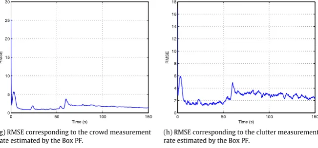
m.

The root mean square error (RMSE) of the box PF and CPF estimates are illustrated in this section. The RMSE values for each time step are calculated over a number of Monte Carlo simulation runs according to

RMSE

=







1

NMC NMC



i=1



x

ˆ

_i

−

x_i



2

,

(55)

where xi represents the ground truth, x

ˆ

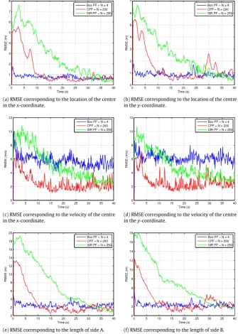
i represents the filter

(9)

(a) RMSE corresponding to the location of the centre in thex-coordinate.

(b) RMSE corresponding to the location of the centre in they-coordinate.

(c) RMSE corresponding to the velocity of the centre in thex-coordinate.

(d) RMSE corresponding to the velocity of the centre in they-coordinate.

[image:9.595.123.459.65.536.2]

(e) RMSE corresponding to the length of side A. (f) RMSE corresponding to the length of side B.

Fig. 2. Comparison of the RMSE for the states of the box PF, CPF and SIR PF with equal computational complexity.

The first set of results illustrate how the box PF, CPF and SIR PF perform when estimating the marginal posterior distribution,

p

(

xk

|

Z1:k

,

λ

k

)

, with measurement and clutter rates assumed

known. Only 4 box particles are required to track the crowd. For comparison, the CPF and SIR PF were also run with 4 particles, however, this resulted in consistent filter divergence due to particle degeneracy. Instead the number of particles were selected based on achieving a similar computational expense for all algorithms. The number of Monte Carlo runs is 100. The resultant RMSE values are illustrated inFig. 2. The comparison of the computational complexity for these results are presented

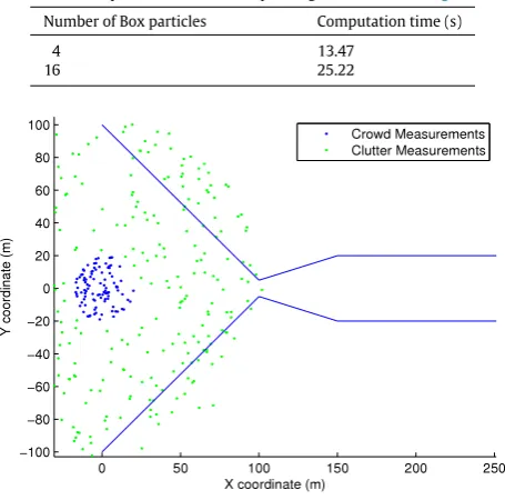
in Table 4. It is worth noting that the implementation of

the box PF utilises the INTLAB toolbox for performing interval operations. INTLAB was initially designed and optimised for estimating rounding errors. We believe that utilising alternative methods for the interval operations could significantly reduce the computational complexity of the box PF. The box PF and CPF are

able to lock on to the crowd significantly faster than the SIR PF. It is noted that the RMSE is generally higher for the box PF once all filters have locked onto the crowd. This can be attributed to the approximations made in the derivation of the marginal posterior pdf. The SIR PF is also matched in terms of the model noise and likelihood expression.