Sparse model identification using a forward orthogonal regression algorithm aided by mutual information

This is a repository copy of Sparse model identification using a forward orthogonal

regression algorithm aided by mutual information.

White Rose Research Online URL for this paper:

http://eprints.whiterose.ac.uk/74559/

Monograph:

Billings, S.A. and Wei, H.L. (2006) Sparse model identification using a forward orthogonal

regression algorithm aided by mutual information. Research Report. ACSE Research

Report no. 919 . Automatic Control and Systems Engineering, University of Sheffield

[email protected] https://eprints.whiterose.ac.uk/

Reuse

Unless indicated otherwise, fulltext items are protected by copyright with all rights reserved. The copyright exception in section 29 of the Copyright, Designs and Patents Act 1988 allows the making of a single copy solely for the purpose of non-commercial research or private study within the limits of fair dealing. The publisher or other rights-holder may allow further reproduction and re-use of this version - refer to the White Rose Research Online record for this item. Where records identify the publisher as the copyright holder, users can verify any specific terms of use on the publisher’s website.

Takedown

If you consider content in White Rose Research Online to be in breach of UK law, please notify us by

S.A. Billings and H.L. Wei

Research Report No. 919

Department of Automatic Control and Systems Engineering

The University of Sheffield

Mappin Street, Sheffield,

S1 3JD, UK

March. 2006

Sparse Model Identification Using A Forward Orthogonal

Regression Algorithm Aided by

2

Abstract—A sparse representations, with satisfactory approximation accuracy, is usually desirable in any nonlinear

system identification and signal processing problem. A new

forward orthogonal regression algorithm, with mutual

information interference, is proposed for sparse model

selection and parameter estimation. The new algorithm can be

used to construct parsimonious linear-in-the-parameters

regression models.

Index Terms—model selection, mutual information, orthogonal least squares, parameter estimation, radial basis

function networks.

I. INTRODUCTION

he central task in learning from data is how to identify a

suitable model from the observational data set. One solution is

to construct nonlinear models using some specific types of

basis functions, aided by various state-of-the-art techniques

[1]-[5]. Among the existing sparse modeling techniques,

linear-in-the-parameters regression models, which will be

considered in the present study, are an important class of

representations for nonlinear function approximation and

signal processing. A general routine for linear-in-the-

parameters modeling often starts by constructing a model term

dictionary

D

, whose elements are the candidate model terms

(1)(2) Department of Automatic Control and Systems Engineering, University of Sheffield, Mappin Street, Sheffield, S1 3JD,UK.

(also called bases) that are formed using some given primary

basis functions according to some specified rules. A dictionary

often contains a large or even an infinite number of candidate

model terms (bases). The task of system identification

involves two aspects: the selection of the significant model

terms and the determination of the number of model terms

involved in the final identified model. The objective is to

obtain a satisfactory sparse representation that involves only a

few bases, by making a compromise between the

approximation accuracy and the model complexity (model

size). Notice that the objective of dynamical modeling is not

merely data fitting. In dynamical modeling the resulting sparse

model should fit the observational data accurately, but at the

same time the model should be capable of capturing the

underlying system dynamics carried by the observational data,

so that the resulting model can be used in simulation, analysis,

and control studies.

Many approaches have been proposed to address the

model structure selection problem, most of these focus on

which bases are significant and should be thus included in the

model. The orthogonal least squares (OLS) algorithm

[2][6][7], which was initiated for nonlinear system

identification, has become popular and has been widely used

for sparse data modeling. This type of algorithm is simple to

Sparse Model Identification Using A Forward Orthogonal

Regression Algorithm Aided by

Mutual Information

Stephen A. Billings

1

and Hua-Liang Wei

2

linear-in-the-parameters models with good generalization

performance [14]. An advantage of the OLS type algorithms is

that commonly used model selection and regularization

techniques, for example the AIC, BIC and cross-validation

(GCV) [8]-[10], can easily be adopted and incorporated into

the model structure selection algorithms to yield compact

linear-in-the- parameters regression models with good

generalization properties [11]-[13].

In the OLS type algorithms, the criterion that is used to

measure the significance of the candidate bases (model terms)

is the error reduction ratio (ERR), which is equivalent to the

squared correlation coefficient and is similar to the commonly

used Pearson correlation function. Experience has shown that

the OLS algorithms interfered by the ERR criterion can

usually produce a satisfactory sparse model with good

generalization performance. The adoption and the domination

of the ERR criterion in the OLS algorithm, however, does not

exclude other criteria. It follows from practical experience that

the selected model subsets are often criterion-dependent

providing that the given model term dictionary is

under-complete (inunder-complete).

In this study, a new criterion, derived from mutual

information, is adopted into the OLS algorithm to measure the

significance of candidate bases and to interfere with the model

subset selection. The motivation of the adoption of a mutual

information criterion is based on the following considerations.

It is known that the task of modeling from data is generally

structure-unknown and the model term dictionary is often

pre-specified and thus fixed. For this case, the selected model

the mutual information criterion and the ERR criterion may or

may not produce exactly the same model structure given the

same modeling problem. The two criteria can be used in

parallel, and the performance of the resultant models can then

be compared. The model with the better performance will be

chosen as the final model. In this manner, the two criteria will

complement each other and thus produce a better model that

may have been achieved using only one signal criterion.

II. The Linear-In-The-Parameters Representation

Consider the identification problem for nonlinear systems

given N pairs of input-output observations,

N t

t

y

t

u

(

),

(

)}

1

{

= .Under some mild conditions a discrete- time

nonlinear system can be described by the following NARX

model [1]

)

(

))

(

,

),

1

(

),

(

,

),

1

(

(

)

(

t

f

y

t

y

t

n

u

t

u

t

n

e

t

y

=

−



−

y

−



−

u

+

(1)

where

u

(t

)

,

y

(t

)

and

e

(t

)

are the system input, output and

noise variables;

n

_uand

n

_y are the maximum lags in the input

and output, respectively; and f is some unknown nonlinear

mapping. It is generally assumed that

e

(t

)

is an independent

identical distributed noise sequence.

The central task of system identification is to find a

suitable approximator

fˆ

for the unknown function f from the

observational data set. One solution is to construct nonlinear

models using some specific types of basis functions including

polynomials, kernel basis functions and multiresolution

wavelets[3]-[6][15]. Among these existing sparse modeling

4

will be considered in the present study, are an important class

of representations for nonlinear function approximation and

signal procession, because compared to nonlinear-in-the-

parameters models, linear-in-the-parameters models are

simpler to analyze mathematically and quicker to compute

numerically.

Let

d

=

n

_y

+

n

_u and

x

(

t

)

=

[

x

1

(

t

),



,

x

_d

(

t

)]

Twith









+

≤

≤

+

−

−

≤

≤

−

=

u y y y y k

n

n

k

n

n

k

t

u

n

k

k

t

y

t

x

1

))

(

(

1

)

(

)

(

(2)

A general form of the linear-in-the-parameter regression

model is given below:

)

(

))

(

(

ˆ

)

(

t

f

t

e

t

y

=

x

+

(

(

))

(

)

1

t

e

t

M m m m

+

=

∑

=

x

φ

θ

)

(

)

(

t

e

t

T

₊

=

(3)

where M is the total number of candidate regressors,

))

(

( t

m

x

φ

(m=1,2, …, M) are the model regressors and

θ

_mare

the model parameters, and

(

t

)

=

[

φ

₁

(

x

(

t

)),



,

φ

_M

(

x

(

t

))]

T

and are the associated regressor vector and parameter

vector, respectively.

III. Mutual Information Interference for Model Structure Selection

In the standard OLS algorithm [2][6][7], the significance

of candidate model terms are measured using the values of

ERR, which is defined as the non-centralized squared

correlation coefficient between two associated vectors. This

coefficient between two given vectors x and y of size N is

defined as

∑

∑

∑

= = =

=

=

_N i i N i i N

i i i

T T T

y

x

y

x

C

1 2 1 2 1 2

2

₍

₎

)

)(

(

)

(

)

,

(

y

y

x

x

y

x

y

x

(4)

Similar to the commonly used standard Pearson correlation

coefficient in statistics, the function in (4) reflects the linear

relationship between two vectors x and y. Both the standard

Pearson correlation coefficient and the squared correlation

coefficient in (4) have wide application in various fields.

Another useful criterion, derived from mutual information,

can be used to measure the relationship of two random

variables by calculating the amount of information that the

two variables share with each other. Mutual information based

algorithms have in recent years been widely applied in various

areas including feature selection [16]-[19]. In the present

study, mutual information will be introduced to form a

complementary criterion to the ERR criterion to interfere with

the model structure selection procedure.

A. Mutual Information

Following [20], mutual information is defined as follows.

Consider two random discrete variables x and y with alphabet

X

and

Y

, respectively, and with a joint probability mass

function p(x, y) and marginal probability mass functions

)

(x

p

and

p

( y

)

. The mutual information

I

( y

x

,

)

is the

relative entropy between the joint distribution and the product

distribution

p

(

x

)

p

(

y

)

, given as

























=

)

(

)

(

)

,

(

log

)

,

(

y

x

y

x

y

x

p

p

p

E

I













=

∑∑

∈ ∈

(

)

(

)

)

,

(

log

)

,

(

y

p

x

p

y

x

p

y

x

p

x Xy Y

(5)

The mutual information

I

( y

x

,

)

is the reduction in the

uncertainty of y due to some knowledge of x, and vice versa.

Mutual information provides a measure of the amount of

regressor in a linear model,

I

( y

x

,

)

can be used to measure the

coherency of x with y in the model.

B. Model Structure Selection with Interference of Mutual Information

Let

y

=

[

y

(

1

),



,

y

(

N

)]

Tbe a vector of measured outputs

at N time instants, and _m

=

[

φ

_m

(

1

),



,

φ

_m

(

N )]

T be a vector

formed by the mth candidate model term, where m=1,2, …, M.

Let

D

=

{

1

,



,

M

}

be a dictionary composed of the M

candidate bases. From the viewpoint of practical modeling and

identification, the finite dimensional set

D

is often redundant.

The model term selection problem is equivalent to finding a

full dimensional subset

{

,

,

}

{

,

,

}

1

1 n i i_n

n

=



=



D

of n

(

n

≤

M

)

bases, from the library

D

, where

k i

k

=

,

}

,

,

2

,

1

{

M

i

_k

∈



and k=1,2, …, n, so that

y

can be

satisfactorily approximated using a linear combination of

n

,

,

,

2

1



as below

e

y

=

θ

_{1 1}

+



+

θ

_{n n}

+

(6)

or in a compact matrix form

e

A

y

=

+

(7)

where the matrix

A

=

[

1

,



,

n

]

is assumed to be of full

column rank,

=

[

θ

1

,



,

θ

_n

]

T is a parameter vector, and

e

is

the approximation error.

The model structure selection procedure starts from

equation (3). Let

r

0

=

y

, and

)}

,

(

{

max

arg

0 1 1 j M

j≤

I r

≤

=



(8)

(5). The first significant basis can thus be selected as

1

1

=

 , and the first associated orthogonal basis can be

chosen as

1

1 

q

=

. Set

1 1 1 1 0 0 1

q

q

q

q

r

r

r

_T T

−

=

(9)

In general, the mth significant model term can be chosen

as follows. Assume that at the (m-1)th step, a subset

D

_m−1,

consisting of (m-1) significant bases, ₁

,

₂

,



,

m₋₁, has

been determined, and the (m-1) selected bases have been

transformed into a new group of orthogonal bases

1 2

1

,

q

,

,

q

m−

q



via some orthogonal transformation. Let

∑

− =

−

=

1 1 ) ( m k k k T k k T j j m j

q

q

q

q

q

(10)

)}

,

(

{

max

arg

1 ( ) 1 1 , m j m m k j m

I

k

q

r

₋ − ≤ ≤ ≠

=





(11)

where _j

∈

D

−

D

_m−1, and

r

_m−1 is the residual vector obtained

in the (m-1)th step. The mth significant basis can then be

chosen as

m

m

=

 and the mth associated orthogonal basis

can be chosen as _m (m) m



q

q

=

. The residual vector

r

_m at the

mth step is given by

m m T m m T m m m

q

q

q

q

r

r

r

1 1 − −

−

=

(12)

Subsequent significant bases can be selected in the same way

step by step. From (12), the vectors

r

_mand

q

_m are orthogonal,

thus m T m m T m m m

q

q

q

r

r

r

2 1 2 1

2

(

)

||

||

||

||

=

₋

−

− (13)

By respectively summing (12) and (13) for m from 1 to n,

6

n n m m m T m m T

m

_q

_r

q

q

q

r

y

∑

= −

₊

=

1

1 ₍₁₄₎

∑

= −

−

=

n m m T m m T m n 1 2 1 2

2

(

)

||

||

||

||

q

q

q

r

y

r

(15)

Notice that if the function

I

(

⋅

,

⋅

)

in (8) and (11) is replaced by

the squared correlation coefficient defined by (4), the above

algorithm then belongs to the class of orthogonal least squares

type algorithms [2][6][7]. The forward orthogonal regression

algorithm interfered with mutual information will be referred

to as the FOR-MI algorithm.

The residual sum of squares,

||

r

n

||

2,which is also known

as the sum-squared-error, or its variants including the

mean-square-error (MSE), can be used to form criteria for model

selection. The model term selection procedure can be

terminated when some specified termination conditions are

met. In the present study, the following GCV criterion

[10][12] is used to determine the model size

)

MSE(

)

GCV(

2

k

k

N

N

k













−

=

N

k

N

N

k 2 2

||

|| r













−

=

(16)

The selection procedure will be terminated at the step where

the index function GCV(k) is minimized.

C. Parameter Estimation

It is easy to verify that the relationship between the

selected original bases 1

,

2

,



,

_m , and the associated

orthogonal bases

q

₁

,

q

₂

,



,

q

_m, is given by

m m

m

Q

R

A

=

(17)

where

R

_m is an

m

×

m

unit upper triangular matrix whose

entries

u

ij

(

1

≤

i

≤

j

≤

m

)

are calculated during the

orthogonalization procedure, and

Q

_m is an

N

×

m

matrix

with orthogonal columns

q

₁

,

q

₂

,



,

q

_m . The unknown

parameter vector, denoted by _m

=

[

θ

1

,

θ

2

,



,

θ

_m

]

T, for the

model with respect to the original bases (similar to (6)), can be

calculated from the triangular equation R_{m m}=g_m with

T m m

=

[

g

1

,

g

2

,



,

g

]

g

, where

(

1

)

/(

k

)

T k k T k k

g

=

r

₋

q

q

q

or

)

/(

)

(

k T k k T k

g

=

y

q

q

q

.

Note that some tricks can be used to avoid selecting

strongly correlated model terms. Assume that at the mth step,

a subset

D

_m, consisting of m significant bases, 1

,

2

,



,

_m,

has been determined. Also assume that _j

∈

D

−

D

_m is

strongly correlated with some bases in

D

_m, that is, _j is a

linear combination of 1

,

2

,



,

_m. Thus,

(

)

0

) ( )

( m

₌

j T m

j

q

q

.

In the implementation of the algorithm, the candidate basis

m

j

∈

D

−

D

will be automatically discarded if

δ

<

) ( ) (

)

(

q

_jm T

q

_jm , where

δ

is a positive number that is

sufficiently small. In this way, any severe mullticolinearity or

ill-conditioning can be avoided.

V. Numerical Example

Example 1. A nonlinear time series was described by the

following model

)

1

(

25

.

0

)

(

t

=

y

t

−

y

) ( )] 2 ( 5 . 0 2 exp[ 20 ) 1 (

cos

π

yt  − y2 t− +

ξ

t

  



 −

+ (18)

where

ξ

(

t

)

~

N

(

0

,

0

.

025

2

)

. By setting the initial value to be

y(0)=0 and y(1)=0, this model was simulated and 1000 data

points were collected. The first 500 points were used for

network training and the remaining 500 data points were used

[image:8.612.330.528.151.315.2]

Fig. 2 The first return maps generated from the identified RBF network models produced by the FOR-MI algorithm, 1000 data points were used to form the return maps. (a) is for the original noise-free time series, with

ξ

(t

)

=0 in (18) and with initial value y(0)=0 and y(1)=0; (b) is for

the FOR-MI identified model with initial value

ˆy

(

0

)

=0 and

ˆy

(

1

)

=0. the noisy observations. The RBF network model adopted the

Gaussian kernel function of the form

















−

−

+

−

−

−

=

₂

2 2 , 2

1

,

]

[

(

2

)

]

)

1

(

[

exp

)

(

σ

φ

m m

m

c

t

y

c

t

y

t

(19)

where the candidate centers

c

_m

=

[

c

_m,1

,

c

_m,2

]

T (m=1,2, …,

498) were chosen to be all the 498 training data points

T

t

y

t

y

t

)

[

(

1

),

(

2

)]

(

=

−

−

x

for t from 3 to 500, and the kernel

width was chosen to be

σ

=

2

.

5

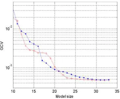
. Both the FOR-MI algorithm

and the OLS-ERR algorithm were applied to the 496 candidate

basis functions. The associated criterion GCV given by (16) is

shown in Fig. 1, where the GCV values suggest that the

number of basis functions (model terms) for the FOR-MI and

the OLS-ERR identified network models should be chosen as

30 and 31, respectively. Comparisons of the identified model

performance on both the training data set and the validation

data set are shown in Table 1.

Starting from

ˆy

(

0

)

=0 and

ˆy

(

1

)

=0, both the FOR-MI and

the OLS-ERR identified models were simulated, and the

model predicted output of 1000 data points generated from the

two models were compared with the noise-free time series

produced by (18) where

ξ

(t

)

was set to be zero. The model

predicted output (MPO) is defined as

))

2

(

ˆ

),

1

(

ˆ

(

ˆ

)

(

ˆ

t

=

f

y

t

−

y

t

−

y

. Table 1 shows the accuracy of

the model predicted output of the two identified network

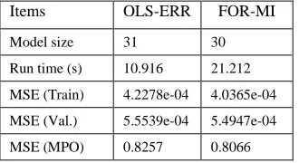
models. It can be seen from Table 1 that the FOR-MI

identified model is slightly superior to the OLS-ERR

identified model for the noisy time series given by (18). A

comparison of the first return map produced from the FOR-MI

by the noise-free model (18), where

ξ

(t

)

was set to be zero, is

shown in Fig. 2.

[image:8.612.325.552.446.617.2]

[image:9.612.91.256.91.181.2]

8

Table 1 Comparison of modelling performance for the OLS-ERR and the FOR-MI identified network models. Items OLS-ERR FOR-MI

Model size 31 30

Run time (s) 10.916 21.212

MSE (Train) 4.2278e-04 4.0365e-04

MSE (Val.) 5.5539e-04 5.4947e-04

MSE (MPO) 0.8257 0.8066

V. Conclusion

To construct sparse models for structure-unknown systems

from observational data, one commonly used approach is to

seek some sparse bases (regressors or model terms) from a

specified dictionary, which may consist of a large number of

candidate bases. Any sparse modeling thus involves the

determination of significant bases. An efficient criterion is

thus needed to measure and rank candidate regressors

according to their significance to the system response. The

criterion ERR is an efficient index to measure the significance

of candidate regressors and is widely used in the OLS type

algorithms for nonlinear model structure selection. The

dominant adoption of the ERR criterion in the OLS algorithm,

however, does not exclude other criteria. It is observed that the

selected model subsets are often criterion-dependent, that is,

the OLS algorithms interfered with by different criteria may

select different significant bases and thus produce different

model subsets. Motivated by this observation, the new

FOR-MI algorithm has been introduced as a complementary

approach to the commonly used least squares type algorithms.

Using the two criteria in a modeling problem may or may not

produce exactly the same model structure. But by inspecting

and comparing the performance of the resulting models, a

more accurate sparse representation can often be obtained. In

this way, the accuracy of the identified sparse model will be

improved compared with results based on any one single

criterion.

REFERENCES

[1] I. J. Leontaritis and S. A. Billings, “Input-output

parametric models for non-linear systems—part I:

deterministic linear systems; part II: stochastic

non-linear systems,” Int. J. Control, vol. 41, no. 2,

pp.303-344, 1985.

[2] S. A. Billings, S. Chen, and M. J. Korenberg,

“Identification of MIMO non-linear systems suing a

forward regression orthogonal estimator,” Int. J. Control,

vol. 49, no.6, pp.2157-2189, June 1989.

[3] S. Chen, and S. A. Billings, “Neural networks for

nonlinear system modelling and identification,” Int. J.

Control, vol. 56, no. 2, pp. 319-346, Aug. 1992.

[4] V. Cherkassky and F. Mulier, Learning from Data. New

York: John Wiley & Sons, 1998.

[5] C.J. Harris, X. Hong, and Q. Gan, Adaptive Modelling,

Estimation and Fusion from Data: A Neurofuzzy

Approach. Berlin : Springer-Verlag, 2002.

[6] M. Korenberg, S. A. Billings, Y. P. Liu, and P. J. McIlroy,

“Orthogonal parameter-estimation algorithm for

non-linear stochastic-systems,” Int. J. Control, vol. 48, no. 1,

pp. 193-210, July 1988.

[7] S. A. Billings, M. J. Korenberg, and S. Chen,

“Identification of non-linear output-affine systems using

an orthogonal least-squares algorithm,” Int. J. Systems

identification,” IEEE Trans. Automat. Contr., vol. 19, pp.

716-723, 1974.

[9] G. Schwarz, “Estimating the dimension of a model,” Ann.

Stat., 6, pp. 461-464, 1978.

[10]G. H. Golub, M. Heath, and G. Wahha, “Generalized

cross-validation as a method for choosing a good ridge

parameter,” Technometrics, 21, pp. 215-223, 1979.

[11]I. J. Leontaritis and S. A. Billings, “Model selection and

validation methods for nonlinear-systems,” Int. J. Control,

vol. 45, no. 1, pp. 311-341, Jan. 1987.

[12]M. J. L. Orr, “Regularization in the selection of radial

basis function centers,” Neural Computation, vol. 7, no. 3,

pp. 606-623, May 1995.

[13]S. Chen, E. S. Chng, and K. Alkadhimi, “Regularized

orthogonal least squares algorithm for constructing radial

basis function networks,” Int. J. Control, vol. 64, no. 5,

pp. 829-837, July 1996.

[14]S.Chen, X. Hong, and C. J. Harris, “Sparse kernel

regression modeling using combined locally regularized

orthogonal least squares and D-optimality experimental

design,” IEEE Trans. Automatic Control, vol. 48, no.6, pp.

1029-1036, June 2003.

[15]S. A. Billings and H. L. Wei, “A new class of wavelet

networks for nonlinear system identification,” IEEE

Trans. Neural Networks, vol. 16, no. 4, pp. 862-874, July

2005.

[16]R. Battiti, “Using mutual information for selecting

features in supervised neural-net learning,” IEEE Trans.

Neural Networks, vol. 5, no. 4, pp. 537-550, July 1994.

networks configuration using mutual information and the

orthogonal least squares algorithm,” Neural Networks,

vol. 9, pp.1619-1637, Dec. 1996.

[18]V. Sindhwani, S. Rakshit, D. Deodhare, D. Erdogmus,

and J. C. Principe, “Feature selection in MLPs and SVMs

based on maximum output information,” IEEE Trans.

Neural Networks, vol. 15, no. 4, pp. 937-948, July 2004.

[19]T. W. S. Chow and D. Huang, “Estimating optimal

feature subsets using efficient estimation of high-

dimensional mutual information,” IEEE Trans. Neural

Networks, vol. 16, no. 1, pp. 213-224, Jan. 2005.

[20]T. M. Cover and J. A. Thomas, Elements of Information