Parallel Simulation of 3D Wave Propagation by Domain
Decomposition
Galina Reshetova1, Vladimir Tcheverda2, Dmitry Vishnevsky2 1
The Institute of Computational Mathematics and Mathematical Geophysics, Siberian Branch of the RAS, Russia 2
The Institute of Petroleum Geology and Geophysics, Siberian Branch of the RAS, Russia Email: [email protected]
Received July 2013
ABSTRACT
In order to perform large scale numerical simulation of wave propagation in 3D heterogeneous multiscale viscoelastic media, Finite Difference technique and its parallel implementation based on domain decomposition is used. A couple of typical statements of borehole geophysics are dealt with—sonic log and cross well measurements. Both of them are essentially multiscales, which claims to take into account heterogeneities of very different sizes in order to provide re-liable results of simulations. Locally refined spatial grids help us to avoid the use of redundantly tiny grid cells in a tar-get area, but cause some troubles with uniform load of Processor Units involved in computations. We present results of scalability tests together with results of numerical simulations for both statements performed for some realistic models.
Keywords: Seismic Wave propagation; Sonic Log; Numerical Simulation; Domain Decomposition
1. Introduction
The most effective way to improve resolving ability of any wave images is to increase dominant frequency of a sounding pulse. But Earth media attenuate and disperse propagating waves. Both these effects are often quanti-fied by the Quality Factor Q. This factor describes rela-tive dissipation of seismic energy per unit volume per unit cycle. If attenuation is not too strong, Quality Factor can be treated as a number of wavelengths a wave can propagate through a medium before its amplitude was decreased in eπ times.
Both fields and laboratory experiments prove that this parameter can be treated as independent on time fre-quency for rather wide frefre-quency range [5]. Therefore the higher is the dominant frequency of a source pulse, the shorter is the distance with reliable level of sig-nal-to-noise ratio. So, in order to get an image with high resolution it is necessary to place acquisition system as close to the target object as possible. The only way to do this is to place sources and/or receivers within boreholes drilled in the vicinity of the target object. In its own turn presence of a well filled with a drilling mud brings es-sential peculiarities to wave fields and should be taken into account in model description. In its own turn, this claims use of locally refined grids in order to catch hete-rogeneities of the smallest scale only.
The paper deals with numerical simulation of waves propagation within viscoelastic media for the following
borehole based geophysical methods:
a) Sonic Log—sources and receivers are within the
same borehole and the main task is monitoring of casing pipe integrity and recovery of near well-bore vicinity. Multiscale nature of the problem becomes apparent in the presence of heterogeneities of at least two different scales-distance source/receiver and borehole radius. If one deals with a cased borehole there is third scale-structure of the casing. Fourth scale can be introduced by a medium;
b) Cross-well Tomography—sources and receivers
are placed within adjacent boreholes encircling a target object. This problem possesses two extremely different scales-borehole diameter and distance between sources and receivers.
2. Viscoelastic Media
Any process of wave propagation within linear elastic medium is governed by two groups of equations:
1) Motion equations (Newton’s law);
2) State equation that connects stress and strain tensors (Hook’s law).
mate-7
rials can be written down in the following way:
( )
(
)
0
( , ) ( , 0 ) ( , ) , ,
ij ijkl kl
t kl
ijkl
x t G x x t
x t
G x d
σ ε ε τ τ τ τ = + ∂ − + ∂
∫
For isotropic viscoelastic materials relaxation tensor simplifies to the following one:
Λ( , ) 2 ( , )
ijkl ij kl ik jl
G =δ δ x t + δ δ M x t
Numerical resolution of integro-differential equations (1) is very troublesome. The most convenient way is to represent state equation in a differential form on a base of mechanical analog of a viscoelastic material like a set of rings and plungers known as Generalized Linear Standard Solid (see [2]). Moreover, real data, both field and laboratory, proved that (see [5-7]): A correct model-ing scheme should yield a constant Quality Factor Q and the corresponding dispersion relation.
The common way to implement these properties of real media in mathematical model is again just men-tioned Generalized Standard Linear Solid (GSLS). For this model the Hook’s law is written down as:
1 ; L j j σ σ = =
∑
ii i MR i
t t
σ σ ε ε
σ τ+ ∂ = ε τ+ ∂
∂ ∂
and introduces Quality Factor as:
2 2 2 1 2 2 1 1 1 1 ( ) ( ) 1
L l l l
l L l l l l L Q σ ε σ ε σ σ ω τ τ
ω τ
ω ω τ τ
ω τ = = + − + + = − +
∑
∑
The problem is how to choose a set of parameters ,
i i
σ ε
τ τ providing desired behavior of Quality Factor over a predefined interval of time frequencies.
We resolve it on the base of Least Squares techniques:
2 1
1 1 2
( , ) | ( ) | min
Jτ τσ ε =
∫
ωω Q− ω −Q− dω→In order to find desired sets of relaxation times we ap-plied τ-method proposed in [1] and modified recently in [3]. Its main advantage is essential reduction of a number of relaxation times-for realistic values of Quality Factor (Q>10) one can manage with single value of τε (and
keep it the same through the target area!) and a couple of
σ
τ . Application of τ -method for GSLS gives the fol-lowing representation of Hook’s law:
1 0
( , ) (1 ) ( , ) 1 ( , ) l R t t L R l l
t x M L t x
M e σ x d
τ τ
σ
σ τ ε
τ ε τ τ
τ − − = = + − −
∑ ∫
Let us differentiate this relation with respect to time
t:
(
) ( )
( )
0( )
1
, 1
1 1
, l ,
R R
t
L t
l l l
t x
M L M
t t
t x e σ x d
τ τ
σ σ
ε
σ τ τ
ε ε τ τ
τ τ − − = ∂ ∂ = + − ∂ ∂ × −
∑
∫
and introduce l-th memory variable
( )
1 0( )
( , ) , l , ]
t t
l R
l l
r t x M t x e σ x
τ τ
σ σ
τ ε ε τ
τ τ
− −
= − −
∫
(2)Straightforward differentiation of (2) provides the fol-lowing equation for this variable:
( , )
l l
R
l l
r v r t x
M
t σ x σ
τ
τ τ
∂ = − ∂ −
∂ ∂
and we come to the following system of first-order PDE for viscoelastic wave propagation:
v t x σ ∂ ∂ = ∂ ∂ 1
(1 ) L
R l l
v
M L r
t x σ τ = ∂ = + ∂ + ∂ ∂
∑
1 l R l l r v M rt τσ x
∂ = − ∂ +
∂ ∂
As one can see, implementation of GSLS claims extra independent “memory” variables per relaxation mechan-ism per stress component. In particular, for 3D models 𝐿𝐿 mechanisms claim 6L new variables besides three dis-placements and six stresses. This leads to significant in-crease of memory demands for simulation of waves’ propagation.
3. Parallel Implementation
Parallel Implementation is based on representation of the area of computations as superposition of disjoints sub-domains touching one another along some contact sur-face. Each of them is assigned to specific Processor Unit (PU). Waves traveling in the model pass through differ-ent subdomains, which require communication between neighboring processors. Essentially different geometry of the target area used in Sonic Log and Cross-hole Tomo-graphy claims necessity of different approaches to Do-main Decomposition (DD) as well. Let us consider both of them.
3.1. Sonic Log
meters. Taking this into account we slice the total 3D model into a number of disc-like subdomains Ω𝑖𝑖. Finite difference scheme assumes communication between neighboring processors requiring them to exchange func-tion values on the interfaces between elementary discs.
It should be noted that DD on the base of this rather simple geometry easily provides possibility to guarantee uniform load of Processor Units involved in computa-tions. Another advantage of the chosen DD is in ex-tremely small portions of data PU should interchange at each time step and, so, extremely small waiting period before computation on the next time step would be done. The MPI (Message Passing Interface) library is applied for arranging the above-mentioned send/receive proce-dures and special efforts are paid in order to minimize idle time of Processor Units due to the data exchange. In order to provide this we start computations for each sub-domain from its interior widening them towards inter-faces and use non-blocking functions Isend and Ireceive
in order to arrange data exchange between neighboring PU.
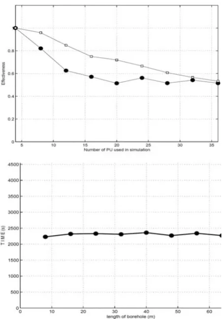
Special attention was paid to analysis of effectiveness and scalability of this approach. This analysis was per-formed by the series of numerical experiments perper-formed on the cluster HKC-160 (Siberian Supercomputer Center, Novosibirsk) made of 80 computation modules (hp Inte-grity rx1620 with two PU Intel Itanium 2, each of 1.6 Ghz, 3 Mb cache, 4 Gb RAM) connected via 24-port commutator InfiniBand (10 Gbot, Cluster Interconnect). Peak performance of the cluster is about 1 Tflop/s. In order to estimate effectiveness of parallelization, fixed computational area was decomposed on different quanti-ty of subdomains, so simulation was performed for the same target area, but with increasing number 𝑛𝑛 of PU. For each 𝑛𝑛effectiveness is found as
4 * (4) ( )
* ( )
time eff n
n time n
= (3)
where time n( ) is computer time expended by 𝑛𝑛 PU for simulation. We start with n=4 in order to provide from the very beginning the same amount of data ex-change between adjacent PU. On Figure 1(a)) one can see effectiveness computed for two different lengths of computational area: 12 meters (circles) and 24 meters (rectangles). These results are completely predictable - the less is load of PU the less is effectiveness. It is con-firmed by behavior of both curves - for target area of 24 meters the load of single PU is twice as many as for tar-get area of 12 meters and decrease of effectiveness is not so sharp, but finally they become the same.
Now let us perform the series of numerical experi-ments in opposite manner-we fix size of elementary subdomains but increase their quantity proportionally to quantity of PU. This result one can see on Figure1(b))
Figure 1. Scalability by numerical experimentations: Up-per-Effectiveness with fixed computational area; Down- Total time with fixed load of PU.
and certain that the computational time does not change under increase of quantity of PU.
So, we can conclude, that the key parameter is ratio of amount of data being load to each of PU and amount of data it should exchange with its neighbor. The higher is this ratio the higher is effectiveness of parallelization. In particular, if this ratio is fixed it does not matter how many PU are involved in simulation.
3.2. Cross-Hole Tomography
[image:3.595.311.537.82.406.2]9
produced by wide contact surface between adjacent sub-domains which leads to essential loss of parallelization effectiveness. In order to minimize amount of data ex-changed between PU we need to reduce surface area of subdomains under fixed number of grid points per each PU—that is to choose them as close to cubes as possible. Under this approach each PU interchange data with 3/6 neighbors.
4. Numerical Experiments
To conclude the paper let us briefly consider simulation results for a couple of realistic models performed on the previously described cluster HKC-160.
Sonic Log
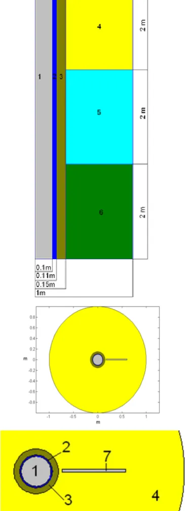
The series of numerical experiments have been imple-mented for a range of source frequencies, positions and models of surrounding elastic media. For illustration let us consider the model with well completion and vertical crack presented on the Figures2 and 3 and possesses the following structure:
1) Vertical borehole with radius 0.1 m filled with a mud with Vp=1500 m/s, =1000 kg/m
3
, Quality Fac-tor Q=65;
2) Steel tube encircling borehole; its width is equal to 0.01 m, wave propagation velocities Vp=5600 m/s,
3270
s
V = m/s, 𝜚𝜚=7830 kg/m3, Quality Factor 100
Q= ;
3) The casing around steel tube; its width is equal to 0.04 m, its elastic parameters are the following: Vp
= 4200 m/s, Vs = 2425 m/s, = 2400 kg/m
3
, Quality Factor Q=80;
4) Background-homogeneous viscoelastic layer with wave propagation velocities Vp = 4989 m/s, Vs =
2605 m/s, = 2400 kg/m3, Quality Factor 100
Q= ;
5) Background-homogeneous viscoelastic layer with wave propagation velocities Vp = 3208 m/s, Vs =
[image:4.595.331.514.97.601.2]1604 m/s, = 2400 kg/m3, Quality Factor Q=60;
Figure 2. Radial and azimuthal grid refinement around well completion.
Figure 3. Upper—Vertical cross-section of the model; Mid-dle—Horizontal cross-section of the model; Down—Zoomed version of Middle figure.
6) Background-homogeneous viscoelastic layer with wave propagation velocities Vp = 2650 m/s, Vs =
1219 m/s, = 2400 kg/m3, Quality Factor Q=15; 7) Vertical crack started at r = 0.18 m and finished at r =
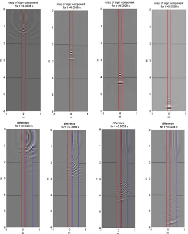
[image:4.595.110.241.573.710.2]
Figure 4. Snapshots for σrr propagating through the plane φ =( , )0π . Left column-the model without crack; Right col-umn-difference between the calculations for the model with and without vertical crack.
during its propagation within borehole and adjacent rocks with and without of vertical crack. There is a series of snapshots for components through the plane ϕ =(0,π) for axial source position with dominant frequency of 10 kHz located in z=0.5 m. Two vertical red lines are projections of interface between borehole and its com-pletion with surrounding rocks, black horizontal lines indicate interfaces of the layers and blue lines follow the crack. The left column figures illustrate wave propaga-tion for the model without of crack, while the right col-umn figures represent the propagation of difference be-tween the wave field with and without of crack.
5. Conclusion
[image:5.595.110.488.84.554.2]11
locally not spatial grid cells only, but time step used for computations as well. Another important axis of devel-opment is connected with necessity to provide an oppor-tunity to perform simulation for more realistic mechani-cal models and above all media with anisotropy induced by fine layering, clusters of microcracks and stresses around a well.
6. Acknowledgements
This work was supported by the Russian Foundation for Basic Research (projects no. 11-05-00947, 13-05-00076 and 13-05-12051).
REFERENCES
[1] J. O. Blanch, J. O. A. Robertsson and W. W. Symes, “Modeling of a Constant Q: Methodology and Algorithm for an Efficient and Optimally Inexpensive Viscoelastic Technique,” Geophysics, Vol. 60, No. 1, 2005, pp. 176-
184.
[2] R. M. Christensen, “Theory of Viscoelasticity—An In-troduction,” Academic Press, Waltham, 1982.
[3] S. Hestholm, et al., “Quick and Accurate Q Parameteriza-tion in Viscoelastic Wave Modeling,” Geophysics, Vol. 71, No. 5, 2006, pp. T147-T150.
[4] V. I. Kostin, D. V. Pissarenko, G. V. Reshetova and V. A. Tcheverda, “Numerical Simulation of 3D Acoustic Log-ging,” Lecture Notes in Computer Sciences, Vol. 4699, 2007, pp. 1045-1054.
[5] F. J. McDonal, F. A. Angona, R. L. Mills, R. L. Sengbush, R. G. van Nostrand and J. E. White, “Attenuation of Shear and Compressional Waves in Pierre Shale,” Geophysics, Vol. 23, No. 3, 1958, pp. 421-439.
[6] S. A. Siddiqui, “Dispersion Analysis of Seismic Data,” M.S. Thesis, University of Tulsa, Tulsa, 1971.
[7] P.C. Wuenschel, “Dispersive Body Waves—An Experi-mental Study,” Geophysics, Vol. 30, No. 4, 1965, pp.