This is a repository copy of
Coronal loop oscillations and diagnostics with Hinode/EIS
.
White Rose Research Online URL for this paper:
http://eprints.whiterose.ac.uk/10683/
Article:
Taroyan, Y. and Bradshaw, S. (2008) Coronal loop oscillations and diagnostics with
Hinode/EIS. Astronomy and Astrophysics, 481 (1). pp. 247-252. ISSN 1432-0746
https://doi.org/10.1051/0004-6361:20078610
[email protected] https://eprints.whiterose.ac.uk/
Reuse
Unless indicated otherwise, fulltext items are protected by copyright with all rights reserved. The copyright exception in section 29 of the Copyright, Designs and Patents Act 1988 allows the making of a single copy solely for the purpose of non-commercial research or private study within the limits of fair dealing. The publisher or other rights-holder may allow further reproduction and re-use of this version - refer to the White Rose Research Online record for this item. Where records identify the publisher as the copyright holder, users can verify any specific terms of use on the publisher’s website.
Takedown
If you consider content in White Rose Research Online to be in breach of UK law, please notify us by
DOI:10.1051/0004-6361:20078610 c
ESO 2008
Astrophysics
&
Coronal loop oscillations and diagnostics with Hinode/EIS
Y. Taroyan
1and S. Bradshaw
21 SP2RC, Department of Applied Mathematics, University of Sheffield, Sheffield S3 7RH, UK e-mail:[email protected]
2 Space & Atmospheric Physics, Blackett Laboratory, Imperial College London, Prince Consort Road, London SW7 2BZ, UK e-mail:[email protected]
Received 4 September 2007/Accepted 17 January 2008
ABSTRACT
Context.Standing slow (acoustic) waves commonly observed in hot coronal loops offer a unique opportunity to understand the prop-erties of the coronal plasma. The lack of evidence for similar oscillations in cooler loops is still a puzzle.
Aims.The high cadence EIS instrument on board recently launched Hinode has the capability to detect wave motion in EUV lines both in the imaging and spectroscopy modes. The paper aims to establish the distinct characteristics of standing and propagating acoustic waves and to predict their footprints in EIS data.
Methods.A 1D hydrodynamic loop model is used and the consequences of various types of heating pulses are examined. In each case, the resulting hydrodynamic evolution of the loop is converted into observables using a selection of available EIS spectral lines and windows.
Results.Propagating/standing acoustic waves are a natural response of the loop plasma to impulsive heating. Synthetic EIS observa-tions of such waves are presented both in the imaging and spectroscopy modes. The waves are best seen and identified in spectroscopy mode observations. It is shown that the intensity oscillations, unlike the Doppler shift oscillations, continuously suffer phase shifts due to heating and cooling of the plasma. It is therefore important to beware of this effect when interpreting the nature of the observed waves.
Key words.Sun: atmosphere – Sun: oscillations – waves – hydrodynamics – line: profiles
1. Introduction
The problem of solar coronal heating first became apparent more than six decades ago. Since then a number of heating theories have been put forward none of which has yet been confirmed. Some of these theories merely represent ideas and concepts. Others are much better developed and involve sophisticated an-alytical and numerical modeling. Solving the coronal heating problem consists of a number of steps which involve their unique problems and challenges. The relationship between these steps is very important. It is easy to forget about the big picture while one is trying to focus on certain isolated aspects of the problem (Klimchuk 2006). A two-way interaction between theories and observations is an important and integral part of solving the heat-ing problem. Such an interaction can only be provided by well developed forward modeling and inversion.
All of the proposed mechanisms require a coupled treatment of dynamically evolving small and large spatial scales which cur-rently poses a severe challenge for multidimensional numerical modeling. Small scales such as current sheets and resonant sur-faces are on the order of meters, whereas large scales such as magnetic loop structures are on the order of mega-meters. As a consequence, the treatment often relies on rather idealized mod-eling. Nevertheless there is still much to be learned even from simple models. A good example are the results of forward mod-eling in 1D (see, e.g., Mariska 1988; Cargill 1993; Hansteen & Wikstol 1994; Reale et al. 1996; Patsourakos & Klimchuk 2006). Using a 1D model and assuming that the heating pro-cess is impulsive, Taroyan et al. (2006) were able to qualitatively reconstruct the average red shifts commonly observed in
transition region lines (see, e.g., Peter & Judge 1999). In re-lation to this problem see also Hansteen (1993).
It is well known that the spectral, spatial and temporal resolu-tion of current space-borne and ground based instruments is lim-ited and this has been a major obstacle for development. Another inhibiting factor which has been somewhat overlooked by theo-reticians is the lack of reliable inversion methods. Among the well-known methods for determining temperature and density profiles along the loops are those based on the analysis of inten-sity ratios which are derived using either imagers or spectrome-ters. The use of such methods has recently been questioned be-cause they have often led to contradictory results (see, e.g., Landi & Landini 2005; Schmelz & Martens 2006). An example illus-trating the existing controversy is a single dataset interpreted in terms of uniform (Priest et al. 1998), footpoint (Aschwanden 2001) and apex (Reale 2002) heating.
MHD waves offer new opportunities for plasma diagnos-tics. Taroyan et al. (2007a) applied a forward modeling ap-proach to confirm the nature of the standing waves seen by SoHO/SUMER, the triggering mechanism and the energies in-volved. Interestingly, standing acoustic type waves have so far been detected only in hot (T > 6 MK) loops. The reason why such oscillations are not seen in cooler loops is still a puzzle. The EIS imaging spectrometer on board the new Hinode satellite could perhaps offer clues due to its high cadence, improved spa-tial resolution and feature tracking capability. One of the main aims of the present followup paper is to predict the footprints of standing and propagating waves in EIS observations. The results are presented both in imaging mode and in spectroscopy mode synthetic observations.
248 Y. Taroyan and S. Bradshaw: Coronal loop oscillations and diagnostics with Hinode/EIS
The presence of individual coherent MHD waves is not guar-anteed. Recently Taroyan et al. (2007b) have proposed a new in-version method which is based on the analysis of power spec-tra for Doppler shift time series. The heating takes place by short-lived pulses which are randomly distributed along the loop. The method could be used to distinguish uniformly heated loops from loops heated at their footpoints and has the potential to de-termine other unique footprints of the actual heating mechanism. The present paper also questions the applicability of the method to intensity times series.
2. 1D loop modeling
In this section the one dimensional loop model is introduced and briefly reviewed. The use of 1D loop models is justified by the fact that the plasma and magnetic field are frozen together and the cross-field thermal conduction is greatly inhibited. The mag-netic field plays only a passive role by channeling the plasma and thermal energy along the field lines. The advantage of using a 1D model is that highly complex field aligned behavior can be accurately simulated using a full energy equation. The disadvan-tage is that the heating must be specified and cannot be computed self-consistently (Klimchuk 2006).
2.1. The governing equations
The plasma motion along a loop is governed by the following set of nonlinear differential equations:
∂ρ ∂t +
∂
∂s[ρv]=0,
∂ ∂t[ρv]+
∂ ∂s[ρv
2]=−∂p
∂s +ρg,
∂e
∂t +
∂
∂s[(e+p)v]=ρvg+H −
∂Fc
∂s − L, (1)
wheresis the coordinate along the loop,ρis density,pis pres-sure,vis velocity,
e= p
γ−1 + ρv2
2 · (2)
is the energy density, g=−g⊙cos
πs
L
(3) is the component of gravitational acceleration along a semicircu-lar loop of lengthL. The right-hand side of the energy equation contains sources and sinks of energy. Any type of heating term Hmust balance the combined thermal and radiative losses. The main losses in the corona. Thermal conduction is expressed in terms of the conductive fluxFc:
Fc=−κT5/2
∂T
∂s, (4)
withκ=10−6erg s−1K−1cm−1being the coefficient of thermal
conduction along the magnetic field. The gradient of conductive flux, i.e., thermal conduction can have both positive and nega-tive values along the loop. It becomes posinega-tive in the lower tran-sition region to balance losses due to strong radiation. The last termL= n2Λ(T) corresponds to optically thin radiative losses wherenis the number density andΛ = Λ(T) is the radiative loss
function. The radiative losses are obtained from a table of values calculated using version 5 of the Chianti atomic database (Dere et al. 1997; Landi et al. 2006), tabulated as a function of tem-perature and density. Thermal bremmstrahlung is also included in the radiation calculation. The ionization balance is assumed to be in equilibrium and has been calculated from the ionization and recombination rates provided by Mazzotta et al. (1998). The element abundances are those due to Feldman (1992).
The chromosphere has an initial depth of 1.5 Mm at each end of the loop and a uniform temperature ofTch = 20 000 K. The chromospheric temperature is maintained against radiative losses using the method described by Klimchuk et al. (1987), where the radiative losses are smoothly decreased to zero over a small temperature interval, dT (100 K in the present work), whereTch ≤ T ≤ Tch+dT. This has the effect of maintaining chromospheric stability such that it may act as a source/sink of mass and energy, while avoiding any significant artificial steep-ening of the radiative loss function at lower temperatures. The boundary conditions are such that the temperature is fixed at 20 000 K and the bulk flow velocity is zero at the edges of the computational domain. We find that the chromosphere in our model is sufficient to damp any significant perturbations that may arise, long before they reach the edges of the domain.
2.2. The role of the transition region
Not including the transition region in the model could result in unphysical coronal solutions to the governing Eq. (1) in the sense that there does not exist a matching solution in the transition re-gion. Further, thermal conduction transfers a large part of the en-ergy deposited in the corona down to the transition region where it is more efficiently radiated due to higher densities and lower temperatures. The transition region is therefore very important for coronal diagnostics and it must be included in the model.
In the subsequent hydrodynamic simulations the heating rate is impulsive, i.e.,H = H(t,s) depends on both time and dis-tance. The transition region moves up and down in response to changing pressure. Not resolving this region properly could pro-duce significant errors in the coronal quantities. It is clear that an adequate treatment of the hydrodynamic evolution of the loop requires an adaptive mesh. In simple terms, points are dynam-ically added in places where they are needed and removed in places where they are no longer necessary. These features are implemented in HYDRAD (Bradshaw & Mason 2003) which is used to integrate the governing Eq. (1).
3. Results
A 30 Mm long loop with an apex temperature of around 1 MK is chosen for the analysis. For simplicity, it is assumed that it has a semicircular shape and no inclination with respect to the vertical plane. The footpoints are anchored in a cool dense chro-mosphere. The loop is initially in hydrostatic equilibrium and a uniform heating ofH0 = 9×10⁻⁴erg cm−3s−1 is applied to balance the losses. The analytical form of the pulse which leads to the formation of a standing wave is given by Taroyan et al. (2005): h= ⎧ ⎪ ⎪ ⎪ ⎨ ⎪ ⎪ ⎪ ⎩
h0sin2 πt
P
exp
−|s−s0| sh
, 0≤t≤P,
0, t>P.
(5)
Such a pulse with a scale length of sh = 2 Mm is applied at
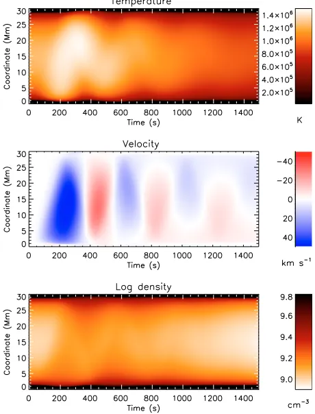
Fig. 1.The hydrodynamic evolution of the loop following a heating pulse near the lower footpoint between 0 s<t<350 s.
s0=1.5 Mm. The main requirement for the formation of a stand-ing wave is that the duration of the pulsePshould be approxi-mately equal to the period of the fundamental mode.
The evolution of temperature, velocity and density along the loop is displayed in Fig.1for the first 1500 s. The impulsive heat deposition increases the temperature of the loop. The pulse has a maximum rate ofh0=2.5×10⁻²erg cm−3s−1and lasts between 0 s and 350 s. The maximum heat flux and total energy input into the loop are 7.5×10⁶erg cm−2s−1 and 9.4×10⁸erg cm−2, respectively. As the transient heating is over, the loop begins to cool due to the combined action of thermal conduction and radi-ation. The fundamental mode period is determined by the ratio of the loop length and the sound speed which is proportional to the square root of temperature. The loop length remains con-stant and therefore the wave period varies because of heating and cooling, i.e., changes in temperature. The time distance diagram for the velocity shows a standing wave pattern which gradually gets deformed as the loop cools to lower temperatures and the os-cillation no longer represents an eigenmode of the system. The velocity oscillation is rapidly damped. The density suffers a tem-porary increase following the injection of heat at the footpoint. Figure2displays the hydrodynamic evolution of the loop when a pulse with a shorter duration is applied at the left footpoint. The heating lasts between 0 s< t <70 s and has a maximum rate ofh0=5×10⁻²erg cm−3s−1. The corresponding maximum heat flux and total energy input into the loop are 1.5×10⁷erg cm−2s−1 and 5.2×10⁸erg cm−2, respectively. The time distance plot for the velocity shows that the pulse propagates back and forth in-side the loop. There are no standing wave patterns like in Fig.1. The total energy injected at the footpoint is smaller compared to the previous case, so the loop cools and the motions vanish faster. Therefore only the first 950 s of the evolution are plotted.
Fig. 2. The hydrodynamic evolution of the loop following a heating
pulse near the lower footpoint between 0 s<t<70 s.
In the next part of the section, the results of hydrodynamic simulations are converted and presented in terms of observable quantities. The details of the applied procedure are described by, e.g., Taroyan et al. (2006).
The EUV imaging spectrometer Hinode/EIS has two CCDs each covering a 40 Å wavelength range: 170–210 Å and 170–210 Å. The wavelength response of EIS has two peaks at around 195 Å and 271 Å corresponding to the two CCDs. The response function is used when synthesizing observables from the simulations. EIS has both narrow (1′′ and 2′′ wide) slits, and wider (40′′ and 266′′) imaging slots, all with 512′′ in the Solar Y direction. EIS should be able to make slit images of ac-tive regions in 10 s, of quiet Sun in between 30 and 60 s, and of flares in approximately one second. The spectral resolution can be less than 3 km s−1 for the Doppler shift. Further details of Hinode/EIS characteristics are given by Culhane et al. (2007), Kosugi et al. (2007).
[image:4.595.40.270.79.381.2]250 Y. Taroyan and S. Bradshaw: Coronal loop oscillations and diagnostics with Hinode/EIS
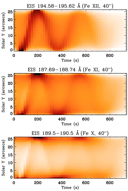
Fig. 3.Synthetic observations of a standing wave by Hinde/EIS in the
imaging mode corresponding to Fig.1. The results are presented in three different wavelengths with a 40′′slot and exposure time of 20 s.
Fig. 4.Synthetic observations of a standing wave by Hinde/EIS in the
spectroscopy mode corresponding to Fig.1. Three different iron lines with a 1′′ slot are used. The black, red and blue lines correspond to Fe
, Fe
and Fe
, respectively.loop is at the disc center and is oriented along the EIS slit in the south-north direction.
[image:5.595.73.281.74.377.2]The results are first presented in the imaging mode. Figure3 shows the synthesized emission in EIS with the 40′′slot. All of the ions which may have a contribution to the emission in the given wavelength range are taken into account. The images are for the standing wave shown in Fig.1. The coordinate in the
Fig. 5.Synthetic observations of a propagating wave by Hinde/EIS in
the imaging mode corresponding to Fig.2. The results are presented in three different wavelengths with a 40′′slot and exposure time of 20 s.
Fig. 6.Synthetic observations of a propagating wave by Hinde/EIS in
the spectroscopy mode corresponding to Fig.2. Three different iron lines with a 1′′slot are used. The black, red and blue lines correspond to Fe
, Fe
and Fe
, respectively.vertical direction is the projection of the loop coordinateson the plane normal to the line of sight:
y= 2L
π sin
2πs
2L
· (6)
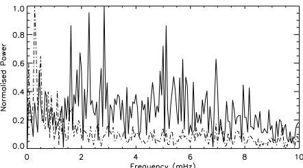
[image:5.595.340.544.425.601.2] [image:5.595.73.279.433.613.2]Fig. 7.Power spectra of the Doppler shift and intensity time series for the Fe
line. The solid and dash-dotted lines correspond to the Doppler shift and the intensity, respectively.temperatures and the oscillation has just begun. The other two windows indicate an oscillatory behavior mainly near the foot-points of the loop. The results of the same hydrodynamic simu-lation are also presented in spectroscopic observations using the 1′′ slit in a sit-and-stare mode. The total intensity of a spectral line is integrated along a 4′′ slit cut from s = 10 Mm down towards the lower footpoint. The choice allows us to study the oscillations both in the intensity and in the Doppler shift. The evolution of the intensity is plotted in the top panel of Fig.4. Arbitrary units have been used by normalizing the intensity with respect to its maximum value. The corresponding Doppler shifts are plotted in the bottom panel. The black, red and blue lines rep-resent Fe
, Fe
and Fe
, respectively. The initial plasma in-flow leads to a positive blue shift which is followed by a damped oscillation. The intensity plots show oscillations superimposed on the background intensity trend. The spectroscopy mode ob-servations indicate oscillatory behavior in all three lines. The quarter period phase shift between the intensity and Doppler shift oscillations seen, for example, in the Fe
during the ini-tial stages of evolution is a well known characteristic of a stand-ing wave (see, e.g., Taroyan et al. 2007a). Figure4shows that the phase of the intensity oscillations undergoes variations in all three lines as it passes through its maximum.A similar procedure is applied to the propagating wave so-lution in Fig.2and the resulting synthetic EIS observations are presented in Fig.5 for the imaging mode and in Fig.6for the spectroscopy mode. The slit/slot selection and the colors used to indicate different lines are the same as those used in Figs.3 and4. It is instructive to compare the synthesized observations of a standing wave with those of a propagating wave. The imaging mode diagrams show that the emission evolves more smoothly in the case of a standing wave. The Doppler peaks are sharper in Fig.6compared to those in Fig.4. The amount of energy re-quired for setting up a standing wave (Fig.4) is almost twice the amount of energy needed for the propagating wave (Fig.6) with a similar amplitude. A comparison between the top and bottom panels of Figs. 4and6 shows that in both cases variations in the phase of the intensity oscillations is present. To further ex-plore this phenomenon, we have simulated impulsive heating of the same loop by random pulses for 5 h. The temperature near the loop apex varies between 0.9 MK and 1.3 MK with an av-erage of about 1 MK. The intensity and Doppler shift time se-ries for Fe
are Fourier analyzed and the resulting power spec-tra are plotted in Fig.7. The solid and dash-dotted lines corre-spond to the Doppler shift and the intensity, respectively. The comparison between the two curves is striking. The power peaksfor the Doppler shift time series are clustered around the fre-quencies of standing wave harmonics (ω ≈2.5,5 mHz) as pre-dicted by Taroyan et al. (2007b). These results are confirmed by the wavelet analysis (not shown). On the other hand, the only significant peak for the intensity time series is located at very low frequencies and is a consequence of the finite duration of the random pulses (<10 s). The peaks corresponding to the nor-mal modes are absent because the intensity oscillations contin-uously suffer phase variations. A mathematical explanation can be given by representing the total intensity as a superposition of a monotonous background and an oscillation:
I(t)=I0(t)+I1cos
2πt P
, (7)
whereI1 is the amplitude of the oscillation and Pis the wave period. As time evolves, the background term I0(t) increases, reaches its peak att0and decreases back. This could represent either cooling or heating of the plasma. Lett−<t0 andt+ >t0 be the positions of any two peaks for the total intensityI(t). We have
I0′(t−)= 2πI1
P sin
2πt−
P
>0, I0′(t+)=2πI1
P sin
2πt+
P
<0. (8) Therefore, the time differenceδt=t+−t−cannot be a multiple of the wave periodP: this would implyI′
0(t−)=I
′
0(t+) whereas, according to Eq. (8), the signs ofI0′(t−) andI0′(t+) are opposite. In other words, the total intensity oscillation undergoes a phase shift whenever the background intensity passes through its peak. In the particular case ofI′0(t−) = −I′0(t+), according to Eq. (8), the phase shift is equal to half a period. Such a behavior is seen, e.g., in the case of the Fe
line in Fig.4.4. Discussion and conclusions
252 Y. Taroyan and S. Bradshaw: Coronal loop oscillations and diagnostics with Hinode/EIS
Both standing and propagating waves are a natural response of the loop plasma to impulsive heating. The results are presented in terms of synthetic EIS observations to predict the wave foot-prints in the actual observations. In the case of imaging mode observations, the waves are most clearly seen in the EIS Fe
195 Å filter when they are just being set up. In contrast to this, the waves clearly appear in all three lines when spectroscopic observations are applied. The quarter period phase shift between the intensity and the Doppler shift oscillations is an indicator of a standing wave. It is shown that the intensity oscillations suffer phase variations when the plasma undergoes heating or cooling. A simple analytical model is used to mathematically explain this phenomenon. Individual coherent MHD waves are not very of-ten seen. Taroyan et al. (2005b) have proposed a new diagnostic method which does not require the presence of such waves. It is based on the analysis of Doppler shift time series and is similar to the approach adopted in helioseismology. The results of the present paper show that this method cannot be successfully ap-plied to the intensity time series because of the phase variations. However, the power spectrum of the Doppler shift time series is quite sensitive to the spatial and temporal distribution of the heating function (Taroyan et al. 2007b). The full potential of this new promising approach has yet to be explored.Acknowledgements. Y.T. is grateful to the Leverhulme Trust for financial sup-port. S.J.B. is grateful to PPARC for their support through the award of a Post-Doctoral Fellowship.
References
Aschwanden, M. J. 2001, A&A, 560, 1035
Bradshaw, S. J., & Mason, H. E. 2003, A&A, 407, 1127 Cargill, P. J. 1993, Sol. Phys., 147, 263,
Culhane, J. L., Harra, L. K., James, A. M., et al. 2007, Sol. Phys., 243, 19 Dere, K. P., Landi, E., Mason, H. E., Monsignori, B. C., & Young, P. R. 1997, A&AS, 125, 149
Feldman, U. 1992, Phys. Scr., 46, 202 Hansteen, V. H. 1993, ApJ, 402, 741
Hansteen, V. H., & Wikstol, O. 1994, A&A, 290, 995 Klimchuk, J. 2006, Sol. Phys., 234, 41
Klimchuk, J. A., Antiochos, S. K., & Mariska, J. T. 1987, ApJ, 320, 409 Kosugi, T., Matsuzaki, K., Sakao, T., et al. 2007, Sol. Phys., 243, 3 Landi, E., & Landini, M. 2005, ApJ, 618, 1039
Landi, E., Del Zanna, G., Young, P. R., et al. 2006, ApJS, 162, 261 Mariska, J. T. 1988, ApJ, 334, 489
Mazzotta, P., Mazzitelli, G., Colafrancesco, S., & Vittorio, N. 1998, A&AS, 133, 403
Ofman, L., & Wang, T. J. 2002, ApJ, 580, L85 Patsourakos, S., & Klimchuk, J. 2006, ApJ, 647, 1452 Peter, H., & Judge, P. G. 1999, ApJ, 522, 1148 Reale, F. 2002, ApJ, 580, 566
Reale, F., Peres G., & Serio S. 1996, A&A, 316, 215
Priest, E. R., Foley, C. R., Heyvaerts, J., et al. 1998, Nature, 393, 545 Schmelz, J. T., & Martens, P. C. H. 2006, ApJ, 636, L49
Taroyan, Y., Erdélyi, R., Bradshaw, S. J., & Doyle, J. G. 2005, A&A, 438, 713 Taroyan, Y., Bradshaw, S. J., & Doyle, J. G. 2006, A&A, 446, 315
Taroyan, Y., Erdélyi, R., Wang, T. J., & Bradshaw, S. J. 2007a, ApJ, 659, L173 Taroyan, Y., Erdélyi, R., Doyle, J. G., & Bradshaw, S. J. 2007b, A&A, 462, 331 Wang, T. J., Solanki, S. K., Curdt, W., Innes, D. E., & Dammasch, I. E. 2002, ApJ, 574, L101