Constructing Compact Dual Ensembles for Efficient Active Learning

Constructing Compact Dual Ensembles for

Efficient Active Learning

Huan Liu1_{, Amit Mandvikar}1_{, and Hiroshi Motoda}2

1_{Department of Computer Science and Engineering, Arizona State University} 2 _{Institute of Scientific and Industrial Research, Osaka University}

{huanliu,amit}@asu.edu, [email protected]

Abstract. A good ensemble is one whose members are both accurate

anddiverse. Active learning requires a small number ofhighlyaccurate

classifiers so that they will not disagree with each other too often. Ensem-ble method, however, are not good candidates for active learning because of their different design purposes. In this paper, we propose to usedual

ensembles for active learning in binary-class domains, and investigate

how to use the diversity of the member classifiers of an ensemble for effi-cient active learning. As active learning requires iterative training of the member classifiers in an ensemble, it is imperative to maintain asmall

number of classifiers in an ensemble for learning efficiency. We empiri-cally show using benchmark data that (1) number of classifiers varies for different data sets to achieve a good (stable) ensemble; (2) feature selec-tion can be applied to classifier selecselec-tion to construct compact ensembles with high performance. A real-world application is used to demonstrate the effectiveness of the proposed approach.

1

Introduction

On the first glimpse, it seems straightforward that ensemble methods can be employed to build classifiers for active learning. A closer look suggests otherwise. This work explores the relationship between the two learning frameworks, at-tempts to take advantage of the good learning performance of ensemble methods for active learning in a real-world application, and studies how to construct an ensemble for effective active learning. In the following, we will first study the relationship between the two in detail in Section 2, propose to use dual ensem-bles for active learning in Section 3, next discuss the diversity issue of ensemble learning with respect to ensemble size - the number of member classifiers in an ensemble as well as empirical results on the benchmark data sets in Section 4, and then go into details of selecting the necessary and diverse member classifiers for an ensemble in Section 5. The experimental results and discussions of active learning with dual ensembles are presented in Section 6. The work is concluded in Section 7.

2

Ensembles and Active Learning

Active learning aims to reach high performance using as few labeled instances as possible. It can be very useful where there are limited resources for label-ing data, and obtainlabel-ing these labels is time-consumlabel-ing or difficult [22]. There exist widely used active learning methods. Some examples are: Uncertainty sam-pling [15] selects the instance on which the current learner has lowest certainty; Pool-based sampling [17] selects the best instances from the entire pool of un-labeled instances; and Query-by-Committee [10, 23] selects instances that have high classification variance themselves. Query-by-Committee (QBC) measures the variance indirectly, by examining the disagreement among class labels as-signed by a set of classifier variants, sampled from the probability distribution of classifiers that results from the labeled training instances. Now let us turn to ensemble methods that also involve building a set of classifiers.

consider Bagging in this work as it is the most straightforward way of manipu-lating the training data [7]. Bagging relies on bootstrap replicates of the original training data to generate multiple classifiers that form an ensemble. Each boot-strap replicate contains, on the average, 63.2% of the original data, with several instances appearing multiple times.

After reviewing an active learning method QBC and an ensemble method Bagging, we notice that both employ a set of classifiers of the same type: active learning uses the set of classifiers to find instances that the classifiers disagree about their predictions, but ensemble learning is to use the set of classifiers to increase diversity in order to achieve high predictive accuracy. Both count on disagreement or diversity of classifiers. Disagreement is closely associated with diversity. Classifiers that do not disagree are not diverse, in other words, only diverse classifiers will possibly disagree. Accuracy and diversity are, however, contradictory goals: diverse classifiers have to make errors on different instances; and accurate classifiers will agree with each other [11]. For example, if a classifier is 100% accurate, other equally accurate classifiers are impossible to disagree, no matter how many of them are generated.

Disagreement or diversity of classifiers are used for different purposes for the two learning frameworks: in ensemble learning, diversity of classifiers is used to ensure high accuracy by voting; in active learning, disagreement of classifiers is used to identify critical instances for labeling. For the former, we want as high diversity as possible; for the latter, disagreement should not occur too often as frequent disagreement requires more manual labeling. In order for active learning to work effectively, we need asmall1_{number ofhighlyaccurate classifiers so that}

they will disagree with each other, but not too often (this is determined by the nature of highly accurate classifiers). Otherwise, the purpose of active learning to learn with as few instances as possible cannot be achieved. For ensemble learning to work, however, one should shun highly accurate classifiers in order to achieve high diversity - weak learners can exhibit high diversity as we discussed earlier - with alargenumber of classifiers. Another essential difference between the two is that active learning is an iterative process and ensemble learning is not. Hence, ensemble learning such as Bagging cannot be simply employed for active learning like QBC.

Since ensemble methods have shown their robustness in producing highly accurate classifiers and each of member classifiers such as decision trees [5, 4, 19] can be very efficient in training and testing, we investigate below (1) how we can employ ensembles in active learning and (2) how we can build compact ensembles for efficient active learning.

3

Dual Ensembles for Active Learning

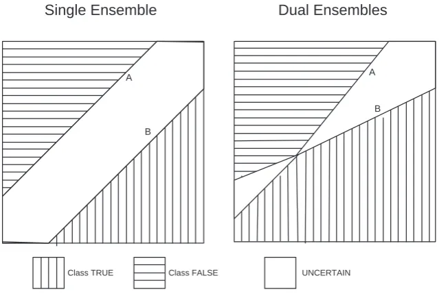
Dual ensembles are class-specific: one ensemble is built for each class in a binary class domain. For a single ensemble to be used in active learning, we need to 1 _{A small ensemble size will make iterative learning more efficient, other things being}

determine two thresholds:δ0 and δ1 to define the majority for classes 0 and 1.

That is to define what a majority of prediction is for 0 or 1 separately: if the number of “1” predictions is> δ1, the ensemble outputs 1; else if the number of

“0” predictions is> δ0, then the ensemble outputs 0; otherwise, the ensemble is

uncertain about its prediction. In addition, there could be many ways to define δ0 and δ1 for a reasonably large ensemble size. The dual ensembles only need

one threshold for each ensemble to define majority which is easy to define: given M classifiers, the threshold is(M+ 1)/2. The above difference is illustrated in Figure 1. When dual ensembles (E1, E0) disagree, uncertain predictions ensue.

The disagreement betweenE1andE0occurs when both are certain but suggest

different outcomes, or both are uncertain. Since ensemblesE1andE0are highly

accurate themselves, we do not expect that they frequently disagree. We use E1 and E0 to classify testing data set and select the uncertain instances by

disagreement. We then ask the expert to label these instances and add the labeled instances to the training data. We continue this until there is not adequate performance increase in subsequent iterations.

Single Ensemble

Dual Ensembles

Class TRUE Class FALSE UNCERTAIN A

B

A A

B

B

Fig. 1.Difference between single and dual ensembles. Classification is defined over the attribute space. A and B define decision boundaries

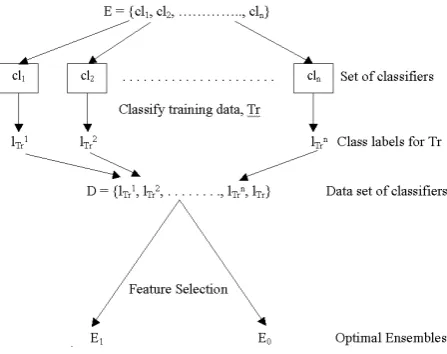
of building dual ensembles in Figure 2. The use of feature selection is discussed in Section 5.

Fig. 2.Procedure to build dual ensembles.

We empirically investigate next whether it is possible to find compact en-sembles with good performance.

4

Accuracy and Diversity of Ensembles

Intuitively, ensemble size required for ensemble learning mainly hinges on the complexity of the training data. For a fixed type of classifier (say, decision trees), the more complex the underlying function of the data is, the more members an ensemble needs. The complexity of the function can always be compensated by increasing the number of members for a given type of classifier until the error rate converges [4, 9]. As we mentioned earlier, an ensemble’s goodness can be measured by accuracy and diversity. Following [11], let ˆY(x) = ˆy1(x), ...ˆy_n(x)

the set of the predictions made by member classifiers C1, ..., C_n of ensemble

E on instance x, y where x is input, and y is the true class. We give some definitions below.

Definition 1. The ensemble prediction of a uniform voting ensemble for inputxunder loss functionl is y(x) =ˆ argmin_y∈Y E_c∈C[l(ˆy_c(x), y].

The ensemble prediction is the one that minimizes the expected loss between the ensemble prediction and the predictions made by each member classifierc for the instancex, y.

The error rate of a data set with N instances can be calculated as e =

1 N

_N

1 LiwhereLi is the loss for instancexi.Accuracyof ensembleEis 1−e.

Definition 3. The diversity of an ensemble on input xunder loss function l is given by D=E_c∈C[l(ˆy_c(x),y(x))].ˆ

The diversity is the expected loss incurred by the predictions of the member classifiers relative to the ensemble prediction. Commonly used loss functions include square loss (l2(ˆy, y) = (ˆy−y)2), absolute loss (l_||(ˆy, y) =|yˆ−y|), and

zero-one loss (l01(ˆy, y) = 0 iff ˆy = y; l01(ˆy, y) = 1 otherwise). In case of a

binary classification problem, these give the same result. We proceed to conduct experiments below.

4.1 Experiments on Benchmark Data Sets

The purpose of the experiments in this section is to observe how diversity and error rate change as ensemble size increases. We use benchmark data sets [1] in the experiments. These data sets have different numbers of classes, different types of attributes and are from different application domains.

We used Weka [24] implementation of Bagging [3] as the ensemble generation method and used J4.8 [24](the Weka’s implementation of C4.5) without pruning as the base learning algorithm in the experiments. For each data set, we run Bagging with increasing ensemble sizes from 5 to 151 and record each ensemble’s error rate e and diversity D. We run 10-fold cross validation and the average values fore andDare calculated.

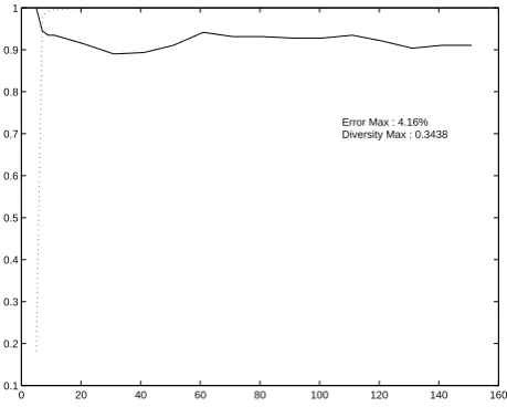
0 20 40 60 80 100 120 140 160 0.1

0.2 0.3 0.4 0.5 0.6 0.7 0.8 0.9 1

Error Max : 4.16% Diversity Max : 0.3438

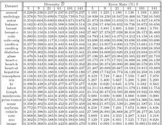
Table 1. Ensemble diversity and error rates for different ensemble sizes on various benchmark data sets.

DiversityD Error Rate (%)e

Dataset

5 9 21 61 101 141 5 9 21 61 101 141

anneal 0.228 0.236 0.237 0.237 0.237 0.237 1.103 1.225 1.180 1.136 1.169 1.203 audiology 0.378 0.701 0.699 0.732 0.739 0.741 18.938 18.230 16.947 16.460 16.726 16.593

autos 0.354 0.604 0.640 0.664 0.671 0.674 21.073 18.098 15.659 15.561 14.927 14.878 balance 0.182 0.455 0.482 0.508 0.508 0.514 18.256 17.456 16.832 16.736 16.672 16.656 breast 0.063 0.341 0.344 0.343 0.343 0.343 4.163 3.891 3.805 3.920 3.863 3.791 breast-c 0.161 0.150 0.159 0.163 0.162 0.164 27.867 27.378 27.028 26.818 26.573 26.469

colic 0.280 0.310 0.328 0.328 0.328 0.328 14.783 14.565 14.375 14.212 14.158 14.185 colic-orig 0.099 0.100 0.117 0.110 0.104 0.101 33.696 33.696 33.696 33.696 33.696 33.696 credit-a 0.357 0.398 0.431 0.442 0.443 0.444 14.261 13.957 14.000 13.725 13.681 13.739 credit-g 0.234 0.252 0.264 0.265 0.265 0.265 27.590 26.450 25.790 25.210 24.930 24.950 diabetes 0.279 0.302 0.338 0.342 0.341 0.341 25.690 24.609 23.620 23.242 23.034 23.073 glass 0.476 0.544 0.592 0.625 0.625 0.637 27.196 25.467 23.084 23.505 22.897 22.710 heart-c 0.300 0.353 0.405 0.432 0.442 0.447 19.175 19.175 17.921 16.898 16.106 16.139 heart-h 0.319 0.343 0.346 0.352 0.351 0.352 20.034 20.374 20.000 20.306 20.578 20.578 heart-st 0.329 0.352 0.394 0.426 0.436 0.437 21.407 20.889 20.667 19.593 19.815 19.889 hepatitis 0.168 0.181 0.180 0.182 0.180 0.180 17.290 17.742 16.774 16.129 16.258 16.129 ionosphere 0.116 0.321 0.327 0.327 0.327 0.327 8.319 7.749 7.464 7.550 7.407 7.379

iris 0.059 0.611 0.624 0.636 0.649 0.652 5.267 5.400 5.667 5.200 5.200 5.200 kr 0.398 0.438 0.473 0.477 0.477 0.477 0.626 0.620 0.645 0.576 0.582 0.563 labor 0.234 0.297 0.325 0.323 0.321 0.319 14.211 13.860 12.281 11.579 11.930 11.754 lymph 0.231 0.396 0.425 0.438 0.440 0.441 21.554 20.473 19.595 20.068 19.932 19.392 mushroom 0.352 0.397 0.431 0.459 0.465 0.472 0.000 0.000 0.000 0.000 0.000 0.000 prim-tumor 0.526 0.700 0.739 0.751 0.752 0.752 58.289 56.873 55.310 54.100 54.366 54.366

sonar 0.358 0.402 0.435 0.452 0.457 0.459 24.904 21.875 21.539 21.298 21.587 21.154 soybean 0.772 0.775 0.824 0.845 0.850 0.853 8.258 7.599 7.291 7.072 6.969 6.838

vehicle 0.231 0.396 0.425 0.438 0.440 0.441 27.589 26.891 26.868 26.277 26.277 26.525 vote 0.068 0.380 0.385 0.384 0.384 0.384 3.609 3.494 3.333 3.287 3.241 3.218

zoo 0.302 0.579 0.588 0.593 0.593 0.593 7.129 7.228 6.931 7.525 7.723 8.020 image 0.318 0.368 0.416 0.442 0.460 0.470 0.093 0.093 0.093 0.095 0.0951 0.0951

4.2 Results and Discussion

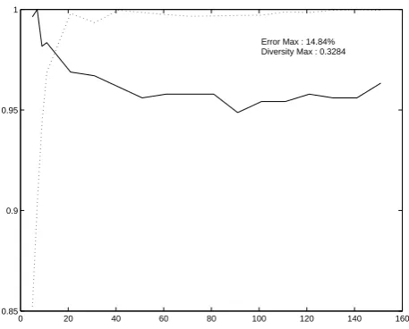
We report diversity and error rates of the sample ensemble sizes (5, 9, 21, 61, 101, 141) in Table 1. The last data set (Image) is from our application domain to be explained later. We have run experiments with 18 ensemble sizes (5, 7, 9, 11, 21, 31, 41, 51, 61, 71, 81, 91, 101, 111, 121, 131, 141, and 151) with 10-fold cross validation for each data set (29 sets in total). Note that for mushroom dataset the error rates are all 0 whereas the diversities are not zero. This is because the error rate becomes 0 if the majority of the member classifiers gives a correct class, even if all of them are not necessarily the same. In Figures 3 and 4, two sets of curves are demonstrated. Both diversity values (dashed lines) and error rates (solid lines) are normalized for plotting purposes. The vertical axis shows percentage (p). The max values of diversity and error rate are given in each figure. We can derive absolute values for diversity and error rates followingMax×p. The trends of diversity and error rates are of our interest. We can observe a general trend that diversity values increase and approach to the maximum, and error rates decrease and become stable as ensemble size increases.

0 20 40 60 80 100 120 140 160 0.85

0.9 0.95 1

Error Max : 14.84% Diversity Max : 0.3284

Fig. 4.Normalized diversity and Error plots for colic data. “1” corresponds to given Max values.

and use these findings for a real-world application on image classification with unlabeled data and propose a novel feature selection approach to choose member classifiers.

5

Selecting Compact Dual Ensembles via Feature

Selection

5.1 Active learning in image domain

The real-world problem we face is to classify Egeria Densa in images. Egeria is an exotic submerged aquatic weed causing navigation and reservoir-pumping problems in the west coast of the USA. As a part of a control program to manage Egeria, classification of Egeria regions in aerial images is required. This task can be stated more specifically as one of classifying massive datawithout class labels. Relying on human experts for labeling Egeria regions is not only time-consuming and costly, but also inconsistent in their performance of labeling. Massive manual classification becomes impractical when images are complex with many different objects (e.g., water, land, Egeria) under varying picture-taking conditions (e.g., deep water, sun glint). In order to automate Egeria classification, we need to ask experts to label images, but want to minimize the task. Active learning is employed to reduce expert involvement in labeling images. The idea is to let experts label some instances of Egeria and non-Egeria regions, learn from these labeled instances, and then apply the active learner to new images. New instances will be recommended by the active learner for labeling, but the number of such instances is expected to be significantly less than labeling all instances in new images. Since experts are still involved in the process of active learning, the retraining with recently requested labeled instances has to be fast so the expert can be actively engaged in the process for high performance classification. Therefore, we need to employ very strong learners (such as ensembles) in order to learn with as few labeled instances as possible. We discuss how to construct dual ensembles for this purpose. Each image consists of 5329 instances (73×73 regions) represented by 13 attributes of color, texture and edge.

5.2 Training data for classifier selection

Often 50-100 member classifiers are used to generate ensembles [4, 20]. They work well for a variety of data sets, as also shown in our benchmark data ex-periments. Since the initial training of ensembles for active learning is off-line, we can afford to choose a larger number. We build our starting ensembleE_max by setting max = 100 member classifiers in this work. The essential problem can be rephrased as: given an ensembleE_max with 100 member classifiers, effi-ciently find a compact ensemble E_M composed of M classifiers, with M being thesmallest number of member classifiers that can have similar error rate and diversity ofE_max.

To generate a training set for the task of selecting member classifiers, we first perform Bagging with 100 member classifiers. We then use the learned classifiers (C_k) to generate predictions for instance x_i, y_i : ˆy_ik = C_k(x_i). The resulting data set consists of instances of the form ((ˆy_i1, ...,yˆ_iK), y_i). After this data set is constructed, the problem of selecting member classifiers becomes one of feature selection.

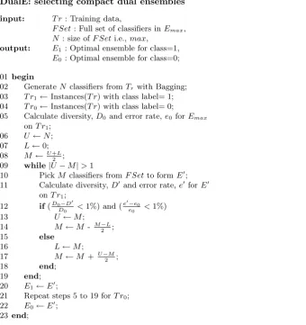
5.3 Algorithm to efficiently determine ensemble size

classifier to be significantly superior to the others. However, when the ensemble size (M) is sufficiently large, accuracy of the members can remain high via voting. Likewise, diversity of an ensemble is also determined by M: an ensemble with a single member has diversity value 0 according to Definition 3. Evidence in the experiments on benchmark data sets suggests that there exists a necessary ensemble size beyond which the performance improvement as the ensemble size increases is not significant.

DualE: selecting compact dual ensembles

input: T r: Training data,

F Set: Full set of classifiers inEmax,

N : size ofF Seti.e.,max,

output: E1 : Optimal ensemble for class=1,

E0 : Optimal ensemble for class=0;

01 begin

02 GenerateN classifiers fromTrwith Bagging; 03 T r1←Instances(T r) with class label= 1; 04 T r0←Instances(T r) with class label= 0;

05 Calculate diversity,D₀ and error rate,e₀forE_max onT r1;

06 U ←N; 07 L←0; 08 M ← U+₂L; 09 while|U−M|>1

10 PickM classifiers fromF Setto formE; 11 Calculate diversity,D and error rate,e forE

onT r1; 12 if(D0−_DD

0 <1%) and ( e−e0

e0 <1%)

13 U ←M;

14 M ←M - M−₂L;

15 else

16 L←M;

17 M ←M + U−₂M; 18 end;

19 end; 20 E1←E;

21 Repeat steps 5 to 19 for T r₀; 22 E0←E;

23 end;

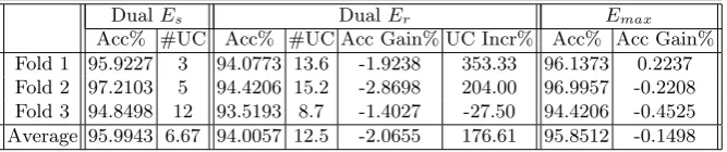
Table 2.Comparison between selected dual ensembles withEmaxfor Breast data

DualEs DualEr Emax

Acc% #UC Acc% #UC Acc Gain% UC Incr% Acc% Acc Gain% Fold 1 95.9227 3 94.0773 13.6 -1.9238 353.33 96.1373 0.2237 Fold 2 97.2103 5 94.4206 15.2 -2.8698 204.00 96.9957 -0.2208 Fold 3 94.8498 12 93.5193 8.7 -1.4027 -27.50 94.4206 -0.4525 Average 95.9943 6.67 94.0057 12.5 -2.0655 176.61 95.8512 -0.1498

Therefore, we only need to determine ensemble sizeM which is the smallest and can keep similar accuracy and diversity of E_max. We design an algorithm DualE that takes O(logmax) to determine M where max is the size of the starting ensemble (e.g., 100)2_{. In other words, we test an ensembleE}

M with size

M which is between upper and lower boundsU andL (initialized asmaxand 0 respectively). IfE_M’s performance is similar to that of E_max, we setU =M andM = (L+M)/2 ; otherwise, setL=M andM = (M +U)/2. The details are in Figure 5. What still remains is the definition of performance similarity between two ensembles. The performance is defined by error rateeand diversity D. The diversity values of the two ensembles are similar if D0−D

D0 ≤pwherepis

a user defined number (0< p <1) for defining similarity (the smaller it is, the more similar) andD0 is of the reference ensemble. In the same spirit, the error

rates of the two ensembles are similar if e−e0

e0 ≤pwheree0 is of the reference

ensemble.

6

Experiments

Two sets of experiments are conducted withDualE: one is on a benchmark data set and the other is on the image data. The purpose is to examine if the compact dual ensembles selected byDualEcan work as expected. When dual ensembles are used, it is possible that they give different class labels to some instances. These instances are calleduncertaininstances. In the context of active learning, the uncertain instances will be given to an expert for labeling. Therefore, the number of uncertain instances is reported in the experiments below in addition to accuracy. For ensemble E_max, the prediction of E_max is the majority of the predictions of the member classifiers, and there is no disagreement. So forE_max only the accuracy is reported and there are no uncertain instances.

6.1 Benchmark data experiment

The classic 10-fold cross validation results of benchmark data sets are in Ta-ble 1. We design a new 3-fold cross validation scheme here, which uses 1-fold for training, the remaining 2 folds for testing. This is repeated for all the 3 folds of

the training data. In addition to comparing with E_max, we also randomly se-lect member classifiers to form dual ensembles. We do so 10 times and use their average accuracy and number of uncertain instances in comparison. The results are shown in Table 2. Average values for each column are also given. Gain (and Incr) is calculated againstE_sas (V−V_Es)/V_Es×100. DualE_sare the selected ensembles usingDualEto ensure that diversity and accuracy of a compact en-semble are similar to E_max. Dual E_r are randomly selected ensembles. Their results averaged over 10 such ensembles are shown in the table. Ensemble sizes of E1 and E0 for ES are 10, 5 for Fold 1; 5, 10 for Fold 2; and 11, 5 for Fold

3, respectively. Ensemble sizes of E1 and E0 for Er are the same as the ones

in E_sfor the corresponding folds. The reduction from 100 to the range of 10 is significant.

Comparing dualE_s and dualE_r, we notice the differences: dual E_r exhibit lower accuracy and higher number of uncertain instances, which manifest the importance of maintaining high accuracy and diversity in building compact en-sembles. Comparing dual E_s and E_max, we observe no significant change in accuracy. This is consistent with what we tried to do in DualE (maintaining both accuracy and diversity). Therefore, selected dual ensembles (E_s) can be used for active learning. The sizes of selected dual ensembles are much smaller than 100 - the size ofE_max.

6.2 Image data experiment

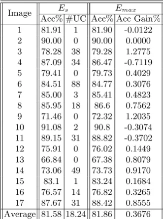
For the image set, there are 17 images already labeled by experts. One image is used for training and the rest for testing. The training results (diversity and error rate) of 10-fold cross validation have been shown in Table 1 (last row). From the viewpoint of active learning, we want to have the training set as small as possible so that in practice, an expert does not need to label too many instances in order to obtain a training data set. The following benchmark data experiment is designed with this purpose in mind. We wish to see if what is learned from one training image can be applied to the remaining images. We first train an initial ensembleE_maxwithmax= 100 on the training image, then obtain accuracy of E_maxfor the 17 testing images. As seen in the last row of Table 1,E_maxis very accurate in terms of 10-fold cross validation. Although images are aerial photos about Egeria, they were shot at different places and times. In other words, these images are similar, but do have their differences from the training image. The idea is to let the learned dual ensembles take care of the majority of the regions of the test images and only recommend the uncertain regions to an expert for labeling, and the labeled instances are used to adapt the dual ensembles.DualE found E1 and E0 of sizes 10 and 5, respectively. Again, they are significantly

Table 3.Selected dual ensembles vs.Emaxfor Image data

Es Emax

Image

Acc% #UC Acc% Acc Gain% 1 81.91 1 81.90 -0.0122 2 90.00 0 90.00 0.0000 3 78.28 38 79.28 1.2775 4 87.09 34 86.47 -0.7119 5 79.41 0 79.73 0.4029 6 84.51 88 84.77 0.3076 7 85.00 3 85.41 0.4823 8 85.95 18 86.6 0.7562 9 71.46 0 72.32 1.2035 10 91.08 2 90.8 -0.3074 11 89.15 31 88.82 -0.3702 12 75.91 0 76.02 0.1449 13 66.84 0 67.38 0.8079 14 73.06 49 73.73 0.9170 15 83.1 1 83.24 0.1684 16 76.57 14 76.82 0.3265 17 87.67 31 88.42 0.8555 Average 81.58 18.24 81.86 0.3676

7

Conclusions

Ensemble methods such as Bagging can achieve good learning performance by increasing ensemble size for high diversity. They have been proven an efficient approach to classification problems. In this work, we point out that (1) ensem-ble methods are not suitaensem-ble for active learning because active learning is an iterative process that interacts with a user for instance labeling; (2) dual en-sembles are very good for active learning if we can build compact enen-sembles. Our empirical study suggests that there exist compact ensembles. We continue to proposeDualEthat can find compact ensembles with good performance via feature selection. Experiments on the benchmark data and image data exhibit the effectiveness of dual ensembles for active learning. We plan to extend dual ensembles to multiple ensembles to handle multi-class classification problems in our future work.

Acknowledgments

References

1. C.L. Blake and C.J. Merz. UCI repository of machine learning databases, 1998. http://www.ics.uci.edu/∼mlearn/MLRepository.html.

2. A. Blum and T. Mitchell. Combining labeled and unlabeled data with co-training.

InCOLT: Proceedings of the Workshop on Computational Learning Theory,

Mor-gan Kaufmann Publishers, 1998.

3. L. Breiman. Bagging predictors. Machine Learning, 24:123–140, 1996.

4. L. Breiman. Random forests. Technical report, Statistics Department, University of California Berkeley, 2001.

5. L. Breiman, J.H. Friedman, R.A. Olshen, and C.J. Stone. Classification and

Re-gression Trees. Wadsworth & Brooks/Cole Advanced Books & Software, 1984.

6. T.G. Dietterich. Machine learning research: Four current directions.AI Magazine, pages 97–136, Winter 1997.

7. T.G. Dietterich. Ensemble methods in machine learning. In First International

Workshop on Multiple Classifier Systems, pages 1–15. Springer-Verlag, 2000.

8. T.G. Dietterich and G. Bakiri. Solving multiclass learning problems via error-correcting output codes. Journal of AI Research, 2:263–286, 1995.

9. Y. Freund and R.E. Schapire. Experiments with a new boosting algorithm. In

Proceedings of the 13th International Conference on Machine Learning, pages 148–

156. Morgan Kaufmann, 1996.

10. Y. Freund, H. Seung, E. Shamir, and N. Tishby. Selective sampling using the query by committee algorithm. Machine Learning, 28:133–168, 1997.

11. M. Goebel, P. Riddle, and M. Barley. A unified decomposition of ensemble loss for predicting ensemble performance. In Proceedings of the 19th International

Conference on Machine Learning, pages 211–218. Morgan Kaufmann, 2002.

12. L. Hans and P. Salamon. Neural network ensembles. IEEE Trans. on Pattern

Analysis and Machine Intelligence, 12:993–1001, 1990.

13. R. Kohavi and G.H. John. Wrappers for feature subset selection. Artificial

Intel-ligence, 97(1-2):273–324, 1997.

14. P. Langley. Selection of relevant features in machine learning. InProceedings of

the AAAI Fall Symposium on Relevance. AAAI Press, 1994.

15. D. Lewis and W. Gale. A sequential algorithm for training text classifiers. In

Proceedings of the Seventeenth Annual ACM-SIGR Conference on Research and

Development in Information Retrieval, pages 3 – 12, 1994.

16. H. Liu and H. Motoda.Feature Selection for Knowledge Discovery & Data Mining. Boston: Kluwer Academic Publishers, 1998.

17. A. McCallum and K. Nigam. Employing EM in pool-based active learning for text classification. InProceedings of the Fifteenth International Conference on Machine

Learning, pages 350–358, 1998.

18. K. Nigam, A. K. Mccallum, S. Thrun, and T. Mitchell. Text classification from labeled and unlabeled documents usingEM. Machine Learning, 39:103–134, 2000. 19. J.R. Quinlan. C4.5: Programs for Machine Learning. Morgan Kaufmann, 1993. 20. J.R. Quinlan. Boosting, bagging, and c4.5. In Proceedings of AAAI, pages 725

–730, 1996.

21. F Roli, G. Giacinto, and G. Vernazza. Methods for designing multiple classifier systems. InMultiple Classifier Systems, pages 78–87. Berlin: Springer-Verlag, 2001. 22. N. Roy and A. McCallum. Toward optimal active learning through sampling esti-mation of error reduction. InProceedings of the Eighteenth International

23. H.S. Seung, M. Opper, and H. Sompolinsky. Query by committee. InProceedings

of the Fifth Annual Workshop on Computational Learning Theory, pages 287–294,

Pittsburgh, PA, 1992. ACM Press, New York.

24. I.H. Witten and E. Frank. Data Mining - Practical Machine Learning Tools and