Single source three dimensional capture of full field plate vibrations

This is a repository copy of

Single source three dimensional capture of full field plate

vibrations

.

White Rose Research Online URL for this paper:

http://eprints.whiterose.ac.uk/79670/

Version: Accepted Version

Article:

Shaw, A.D., Neild, S.A., Wagg, D.J. et al. (1 more author) (2012) Single source three

dimensional capture of full field plate vibrations. Experimental Mechanics, 52 (7). 965 -

974. ISSN 0014-4851

https://doi.org/10.1007/s11340-011-9554-4

[email protected]

Reuse

Unless indicated otherwise, fulltext items are protected by copyright with all rights reserved. The copyright exception in section 29 of the Copyright, Designs and Patents Act 1988 allows the making of a single copy solely for the purpose of non-commercial research or private study within the limits of fair dealing. The publisher or other rights-holder may allow further reproduction and re-use of this version - refer to the White Rose Research Online record for this item. Where records identify the publisher as the copyright holder, users can verify any specific terms of use on the publisher’s website.

Takedown

If you consider content in White Rose Research Online to be in breach of UK law, please notify us by

Experimental Mechanics 52(7):965-974 (2012)

DOI:10.1007/s11340-011-9554-4

Single Source Three Dimensional Capture of Full

Field Plate Vibrations

A.D. Shaw

S.A. Neild

D.J. Wagg

P.M. Weaver

February 2011

Abstract

Measurement of the vibrations of plates can offer significant challenges to the experimentalist, particularly when the plates are lightweight, exhibit large ampli-tude deflections, nonlinear responses or are initially curved. The use of accelerom-eters adds masses which can change the dynamics of lightweight plates. Large am-plitude oscillations and initial curvatures cause complications when using a laser vibrometer, as they make it difficult to get consistent reflections back to the re-ceiver. Furthermore, large or nonlinear oscillations challenge inherent assumptions on which the vibrometer’s algorithms depend. A high speed video camera avoids these issues, but makes it hard to extract numerical data.

This paper describes a method that extends the capabilities of a high speed video camera by using a mirror, allowing post-processing software to stereoscop-ically resolve an array of points on the plate surface to 3D coordinates, capturing the complete shape and position of the plate throughout vibration. This method avoids all the problems mentioned above and gives very clear insight into plate vibration.

Some example results of this method are presented, using thermally bistable carbon laminate plates filmed at a 1000 frames per second. These plates pose the challenges described, and also exhibit an unusual oscillatory motion where the plates ‘snap’ between two statically stable states. The method is shown to provide clear insight into the rich dynamics of these plates.

1

Introduction

physi-cally attaching transducers (usually accelerometers) to the structure that is being anal-ysed, and are well-proven in many contexts [6]. However, when the structure has low mass, such as a thin plate, the additional mass of the attached sensors has an undesirable influence on the system being analysed. Furthermore, practical limits on the number of sensors deployed mean that in general they do not resolve a ‘full field’ deflection shape.

Non-contact methods require little or no attachments to the structure under test, and therefore they avoid the problem of unwanted mass. The predominant example of a non-contact method is the use of the Laser Doppler Vibrometer (LDV), or for full-field measurements, the Scanning Laser Doppler Vibrometer (SLDV). The LDV works by directing laser light at a target on the structure under test, which is reflected back to a receiver that measures the Doppler-shifted wavelength with an interferometer, which is then used to calculate the velocity of the target. A number of instantaneous velocities are measured over a period of time to deduce the resulting vibration. An SLDV extends this by using a controller to perform the test on an array of pre-selected targets, to create a full field measurement. This method is successfully used on a widespread basis [6].

However, there are certain situations where the use of the SLDV proves limiting. One example is the measurement of curved plates; the curvature can mean that light is reflected away from the receiver, leading to poor resolution of the signal. Furthermore, when oscillations become large, there may be significant motion that is in the plane normal to the laser beam. This poses two problems; the first that the vibrometer may not capture the true amplitude of vibration, and the second that the laser target is moving relative to the physical surface of the plate.

A second problem with SLDV tests occurs when complex and nonlinear responses are encountered. The SLDV does not measure each point simultaneously; each point is measured in turn, and then the measured signals are combined to provide a view of the overall deflection motions (an exception to this is the Continuous-Scan LDV as

described by Stanbridgeet al. [14]). The algorithms that perform these calculations

are generally proprietary and not typically available to the researcher; therefore it is unknown whether they are valid in the case of non-linear vibrations, particularly if chaotic motions are encountered. Furthermore, because the LDV is a velocity measur-ing device, there is no true check of the shape of the plate at any given point; the mean point of oscillation is assumed to be the static shape, when this is not necessarily true for nonlinear oscillation.

Another non-contact strategy that can be used is high-speed video. However, on its own this method will only provide a qualitative view of the vibration behaviour.

There is a wide body on stereoscopic imaging systems, that make use of multiple images of a single scene to provide detailed 3D measurements [7, 11]. One approach to stereoscopic imaging is to use mirrors to generate multiple views, saving the com-plexity and cost of additional cameras. This approach also eliminates the need to syn-chronize cameras, although it is penalised by a reduction in the field of view, due to

multiple perspectives being served by one image. Lin et al. [9] and Maet al.[10] have

used multiple mirror systems for the capture of facial motion for the purpose of

com-puter animation. Putzeet al. [13] describes multiple mirror systems combined with

a high speed video cameras, and shows that they can achieve comparable accuracy to

1.

2.

3.

Figure 1: Process of bistable plate manufacture. (1) A flat laminate of directional plies with asymmetric stacking sequence is cured at elevated temperature in an autoclave. (2) On initial cooling the plate distorts into a saddle shape, due to contraction that is asymmetric through its thickness. (3) On further cooling, as curvature increases, the saddle becomes unstable, and the plate adopts one of two possible stable configurations, which it can ‘snap’ between

mirrors to provide an orientable view of a scene [15]. Pankowet al.used a multi-mirror

system to measure deformation of thin plates in response to shocks [12].

This paper outlines a method that extends the use of a high speed digital video camera with just a single mirror. The technique allows the 3D locations of points over the surface of a plate to be recorded in each frame of the video, thereby measuring the full field motion of the plate. It therefore avoids unwanted mass, and makes no assumptions about the nature of the motion being measured. Furthermore, it directly captures shape information. The paper therefore extends the use of stereoscopic vision to gain new insights in the fields of plate dynamics.

To demonstrate the method, the case of a bistable curved laminated plate is consid-ered, which will be described in section 2. Section 3 describes the image capture and data processing method, and Section 5 presents some example vibration responses for bistable plates. Conclusions are drawn in Section 6.

2

Case Study - Curved Bistable Plates

The experiment for which the method was developed was an investigation into the vi-bration mode shapes of bistable carbon composite laminated plates. These are plates made from asymmetric laminates of carbon/epoxy plies which distort on cooling from the cure temperature due to the directional thermal expansion coefficients of the plies [2]. At room temperature they ‘snap’ between two stable configurations [2]. Figure 1 briefly shows how these plates are formed. Such plates have possible applications in morph-ing structures. Their use in such structures is bemorph-ing investigated in order to exploit the property of multiple stable states [3] [4].

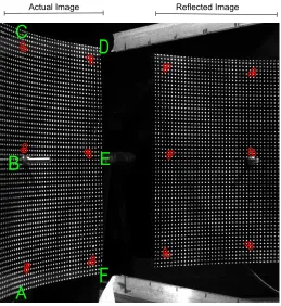
Actual Image Reflected Image

A

B

C

D

E

F

Figure 2: Typical image for processing. Points A-F are reference locations on the surface of the plate, circles show manually selected points for calibration. Note that in this case, only half the plate has been filmed to make best use of the camera resolution; the other half can be inferred in the typical case of symmetric or antisymmetric motion

C

_C'

X

Y

Z

X'

Y'

Z'

Mirror

Plane

True camera image plane

Virtual camera image plane

x

y

x'

y'

f

Physical Point Reflected Point

{t}

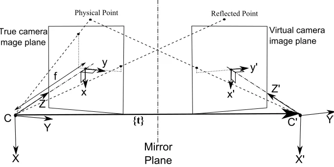
Figure 3: Diagram illustrating the geometric principle of using a mirror for stereoscopic

resolution. The true camera’s focal point atCis the origin of the ‘True camera’

coor-dinate system. The true camera’s projection of the reflected point is a simple reflected transformation of the projection of the physical point in a ‘Virtual camera’ system with

origin at pointC′. Hence the reflection can be used to construct a stereoscopic system,

as if a second camera existed atC′.{t}is the translation vector between the origins of

the two coordinate systems

3

Description of Method

3.1

Overview

A high speed camera is used to record the motion of points on the structure, along with their reflections in an angled mirror which allows post-processing software to resolve 3D locations of points painted on the plate surface. The camera used for the case study was a Photron Fastcam SA1, running at 1000 frames per second.

Figure 2 shows a typical single frame captured by the camera during the case study experiment. The image processing routine traces the 3D location of each dot by using the dot’s reflection to perform a triangulation. To make best use of the camera reso-lution, only half of the plate was filmed for the case study; line AC in Figure 2 is a centreline of the plate. The other half of the plate could be inferred by the symmetry or antisymmetry of the observed deflections.

The stages of this experimental method are:

1. Use our Matlab-based software to calibrate its position with regard to the mirror, as detailed in Section 3.2.

2. Extract 2D image coordinates of points from the images taken, as described in section 3.3.

and triangulate the resulting 3D location, as detailed in Section 3.4 and Section 3.5.

4. Final data transformation and reduction, as described in Section 3.6.

These stages are described in the subsequent sections.

3.2

Calibration

Figure 3 shows the geometry of the method. A simple forward-projection pinhole model is used to represent the camera, and its virtual equivalent. For simplicity we assume that sensor coordinates are unskewed and already transformed into the system

shown asx,y,x′andy′in Figure 3. We also assume that the virtual camera is identical

to the true camera, an assumption that implies that the mirror has no effect on the apparent internal properties of the virtual camera, and therefore both cameras have the

same focal lengthf.

The true camera’s focal pointCis the origin of the ‘true’ coordinate system as

shown in Figure 3, and the virtual camera’s focal pointC′is the origin of the ‘virtual’

coordinate system. Coordinates in the true camera system can be transformed to the virtual coordinate system by means of a simple rotation and transformation;

mathemat-ically ifPandP′represent the same physical point in the true and virtual coordinate

systems respectively we may write:

{P′}= [R]{P}+{t} (1)

where{P}={X,Y,Z}

T

,{P′}={X′,Y

′

,Z

′_}T

, the translation vector{t}={t1,t2,t3}

T

and[R]is the 3D rotation matrix given as:

[R] = 



R11 R12 R13

R21 R22 R23

R31 R32 R33





The task of calibration is therefore to establish[R]and{t}. Note that[R]allows any

3D rotation, and can therefore compensate for any misalignment of the image verticals with the mirror plane.

The calibration process used is a simplified form of the bundled adjustment

pro-cedure as described by Suttonet al. [11], solving for just the rotation and translation

between camera systems. Firstly, using interactive routines from Matlab’s image pro-cessing toolbox [8], the user manually selects a number of corresponding pairs of points from the true and reflected image, as shown in Figure 2. These are grouped in threes so that the local plane can be resolved, which is used in Section 3.4.3. The routines locate the centroidal position of each selected point.

The calibration procedure then minimises a least squares metric based on the dis-tance in each image plane between the sensor coordinates for each point, and the true projections of the 3D point as implied by the given parameters:

E=

N

∑

wherexn,yn andx′n,y′n are the sensor coordinates in the true and virtual image

planes respectively, ˆxn, ˆyn, ˆx′nand ˆy′nare the image plane coordinates projected from the

calculated 3D points, andβ is a vector of the parameters to be tuned. The components

ofβ are given by:

β={n1,n2,n3,t1,t2,t3}

T

(3)

wheren1,n2andn3are components of a vector forming the minimal parametrisation

of[R], where the direction of the vector defines the axis of rotation, and the magnitude

of its angle in radians [11], andt1,t2andt3are components of the translation vector

{t}. Hence to calculate ˆxn(β), the procedure calculates the 3D position of the point

Pnimplied by the true and reflected points and current parameters, using the method

described in Section 3.5, and then evaluates:

ˆ

xn= f

Xn

Zn

, yˆn=f Yn

Zn

(4)

which can be derived graphically from Figure 3. For ˆx′_nand ˆy′_n, the 3D coordinates must

be transformed into the virtual coordinate system using Equation 1 and the calculation is then similar to Equation 4.

E is minimised using a Levenberg-Marquardt solver to perform the nonlinear

op-timisation, where the initial values may be estimated using standard geometry. The

solver was as implemented within the Matlab functionlsqnonlin[8]. Finally, to

provide useful dimensional units to the returned coordinates, a scaling factor for the system is calculated based on known distances between the physical points used for

calibration. Note that in this simple model, focal length f is effectively an arbitrary

scaling factor, which could vary infinitely if{t}varied accordingly, so it is held

con-stant during optimisation.

3.3

Extraction of 2D Positional Data

Matlab’s image processing toolbox routines [8] were used to interactively mask the true image region and the reflected region, to create separate images. The images were then reduced to binary images whereby each pixel is set to either 1 or 0 according to whether

its brightness exceeds a certain threshold, using Matlab functionim2bw. Each dot is

therefore represented as an interconnected region of ones in the grid of pixel values.

Matlab’s functionbwconncompis then used to locate these regions, and the function

regionpropsis used to automatically calculate their centroids. In this manner both the true and reflected images are reduced to simple lists of 2D points on the image plane. The virtual image points are reflected about the central vertical axis, so that the geometry of Figure 3 may be realised.

3.4

Correspondence

• Epipolar constraint

• Ordering

• Surface planarity

• Uniqueness

These are detailed in the following subsections.

3.4.1 Epipolar constraint

This constraint is discussed widely in literature on stereoscopic imaging [7, 11]. As can be seen in Figure 3, the physical point, its projections, both camera origins and the translation vector between them must all lie in a common plane, known as the epipolar plane. Therefore the epipolar planes for all sensor points are resolved using standard vector geometry, and any pairings of true and virtual points where the angles of plane differ outside a certain error tolerance (in this experiment 0.03°) are rejected.

3.4.2 Ordering constraint

The subject of the measurement is a single continuous surface, so therefore it is possi-ble to eliminate many candidate matches based on an ordering constraint as described by Faugeras [7]. The geometrical basis of this constraint is shown in Figure 4. The projected distance of all points onto the direction of the stereoscopic translation vector

{t} is calculated using the dot product. This is then used to sort all true and mirror

points. Hence whenever a correspondence is found with sensor locations{p}and{p′}

in true and virtual image planes respectively, the algorithm finds all true and reflected points within tolerance of their epipolar planes, and eliminates any correspondences

where the true point occurs before{p}and the mirror point after{p′}or vice versa.

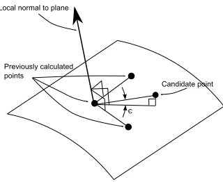
3.4.3 Surface Planarity

This test uses the fact that the test subject is a smooth surface, effectively limiting local surface curvature. Figure 5 illustrates the geometry of the test. A candidate pair of points has its implied 3D position calculated as described in Section 3.5. The algo-rithm then searches for 3 other previously calculated and confirmed points within a 3D zone near this point. It also ensures that these points are not close to being aligned with each another and are not too close to one another, so that they offer good reso-lution of the local surface plane orientation. If this search is successful the algorithm

calculates the angleε as shown in Figure 5 using vector geometry. If this angle is

greater than a specified limitεmax, implying that the point does not appear to lie near to

the local surface plane, the candidate pairing is rejected. For many candidate pairings, this test will initially fail to find nearby points with which to perform the comparison. These points must therefore wait till later passes through the data occur, as described in Section 3.4.5, to be confirmed or rejected by this test.

The 3D zone used in this case was a cubic zone of side 32mm, andεmaxwas set to

C {t} C' Shaker and plate

Mirror Plane True Image

Plane

Virtual Image Plane False point

Figure 4: Diagram showing the principle of the ordering constraint. A collection of points within a single epipolar plane must preserve their order in the direction of the

translation vector{t}in both images. A candidate pairing which does not respect this

ordering will apparently lie in front or behind the surface of other dots, and therefore be false

Local normal to plane

Candidate point Previously calculated

points

Є

Figure 5: Method used to findε to test for point validity. A vector is calculated

be-tween the candidate point and a previously calculated point. The angleεbetween this

3.4.4 Uniqueness constraint

If, for a given true image point, there are multiple pairings with virtual images points that pass all the above constraints, none of these pairings are confirmed as true corre-spondences. Similarly, if multiple true image points pass the above tests when paired with a single mirror image point, none of these pairings are confirmed. This is a conser-vative strategy to handle the case where noise points exist so near to an actual point that the resulting 3D point calculation can still pass other tests. This can cause a true corre-spondence to be rejected along with the ‘noise’ pairing, but with the large numbers of points present in the grid, the numbers of points lost in this way is insignificant.

3.4.5 Overall correspondence algorithm

In the experiment shown there are approximately 2000 visible points in the grid, ap-pearing in each of the true and mirror images, leading to around 4 million candidate pairings. The epipolar constraint is used to filter this list, and typically leaves approx-imately 20000 candidate pairings. The calibration points are then added to the list of confirmed 3D points, and used to reject further pairings based on the ordering con-straint. Then for all remaining candidate pairings:

• If possible, the planarity test is calculated, and candidate pairs that fail are re-jected.

• Any candidate pairs that have passed the planarity test and pass the uniqueness constraint are added to the list of confirmed points, and used to perform further filtering with the ordering constraint.

• This process is repeated for all points until no more pairings are confirmed or rejected.

3.5

Skew Triangulation of 3D Points

The 3D triangulation method is a simple implementation ‘skew triangulation’ method, as described in much of the literature [7, 11]. Referring to Figure 3, the relationship

between a point at{X,Y,Z}

T

in the true camera image system, and its image plane coordinates{x,y}

T

may be written

f X+0Y−xZ=0

0X+f Y−yZ=0 (5)

The same relationship may be written for the virtual camera system and image plane:

f X′+0Y′−x′Z′=0

Substituting Equation (1) into (6) gives:

(f R11−x′R31)X+ (f R12−x′R32)Y+ (f R13−x′R33)Z=−f t1+x′t3

(f R21−y′R31)X+ (f R22−y′R32)Y+ (f R23−y′R33)Z=−f t2+y′t3

(7)

Equations (5) and (7) form an overconstrained set of equations that may be written in matrix form as:

[M]{P}= 

  

M11 M12 M13

M21 M22 M23

M31 M32 M33

M41 M42 M43

       X Y Z    =        0 0

−f t1+x′t3

−f t2+y′t3

      

={r} (8)

This is solved using the generalised inverse as follows:

{P}=[M]T[M]−1[M]T{r} (9)

Therefore Equation (9) is used to calculate the 3D point{P}={X,Y,Z}

T

given

sensor coordinate values for{x,y}

T

and{x′,y

′_}T

, and the stereoscopic rotation matrix and translation vector.

3.6

Data Transformation and Reduction

Generally it will be required to perform a coordinate transformations to find more

use-ful coordinate system, e.g so thatxandyare the approximate plane of the plate andzis

normal to this plane. Then, it will typically be required to calculate 3D displacements, by taking a single image of the plate at rest and subtracting these coordinates from those for each individual frame of the plate in motion.

The Matlab surface fitting toolbox is then used to fit a 5th order polynomial surface to the data [8]. Figure 6 shows two snapshots at opposite peaks of the vertical displace-ment field of a curved plate in a given mode of vibration, including both the actual data points calculated and the smoothed surface. As seen in Figure 6, this fitted surface lies within the noise level of the data in all parts of the plate, and provides much clearer views of mode shapes than a ‘cloud’ of separate dots can provide.

4

Error Analysis

As a means of confirming the accuracy of the method, an error estimation was carried

out using the geometry shown in figure 7, wherePis a point calculated by the routine

with coordinates(X,Y,Z)in the true camera system, (x,y)are its associated sensor

coordinates in the true camera system and(xˆ,y)ˆ is the calculated projection onto the

true image plane using the calibrated model parameters, where:

ˆ

x=X f

Z , yˆ=Y f

−20 0 20 40 60 80 100 120 −100 −50

0 50 100 −2.5

−2 −1.5 −1 −0.5 0 0.5 1 1.5

y /mm x /mm

w /mm

Figure 6: Typical vertical displacement plot at peaks of oscillations, showing quality of polynomial fit

C _C'

X Y Z

X' Y' Z'

Mirror Plane True camera

image plane

Virtual camera image plane (x,y)

(x',y') (x,y)

(x',y')

^

^ ^^

P

x (mm)

y (mm)

−20 0 20 40 60 80 100 120 −100

−50 0 50 100 150

−20 −18 −16 −14 −12 −10 −8 −6 −4 −2 0

Figure 8: Isovalues of vertical heightzof bistable plate, showing subtle doubly curved

regions

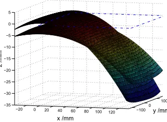
−20 0 20 40 60 80 100 120 −100 0

100 −35

−30 −25 −20 −15 −10 −5 0 5

y /mm x /mm

z

/mm

Figure 9: Shapes of bistable plate at 53Hz, at opposite peaks of oscillation. Dashed lines show the approximate plan area of the half plate

The distancehbetween(x,y)and(xˆ,y)ˆ is readily calculated using Pythagoras

the-orem, and this may be scaled into true dimension units by:

H=hZ

f (11)

An equivalent metricH′can be calculated in the virtual image system.

These variables were calculated for all points in a sample image, and bothHandH′

showed a half-normal statistical distribution, with no apparent geometrical bias around the image, suggesting the dominant source of error was random digitisation noise. The

−20 0 20 40 60 80 100 120 −100

0 100

−5 −4 −3

−2 −1 0 1 2

3 4 5

x /mm

w

/

mm

y /mm

Figure 10: Vertical displacements against initial x-y location of bistable plate at 53Hz,

at opposite peaks of oscillation. (w represents deflection in the verticalzdirection,

relative to the original static shape)

0 0.01 0.02 0.03 0.04 0.05 0.06 −5

0 5

u /mm

0 0.01 0.02 0.03 0.04 0.05 0.06 −5

0 5

v /mm

0 0.01 0.02 0.03 0.04 0.05 0.06 −5

0 5

w /mm

t /s

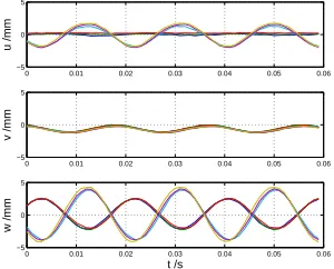
Figure 11: 3D time traces from approximate locations points A-F as shown in Figure

2, showing significant horizontal motion. (u,vandwrepresent displacement in the

−5 0 5

t = 0.012 s

−5 0 5

t = 0.018 s

−5 0 5

t = 0.023 s

−5 0 5

t = 0.029 s

−5 0 5

t = 0.035 s

−5 0 5

t = 0.042 s

−5 0 5

t = 0.048 s

−5 0 5

t = 0.054 s

−5 0 5

t = 0.059 s

−5 0 5

t = 0.065 s

−5 0 5

t = 0.071 s

−5 0 5

t = 0.077 s

Figure 12: 3D sequence of plate snapping at 40.3Hz excitation. The first 3 frames show the plate snapping between stable states, then frames 4 to 6 show a small oscillation without snapping. Frames 7 to 9 show the plate snapping back, and frames 10 to 12 show another small oscillation before the sequence repeats. Frames 2 and 8 show that the plate forms a saddle configuration when midway through a snapping motion. Note

5

Results from Case Study

This section presents some results from a case study experiment that highlights the insight that this method can give.

5.1

True Static Shape of Bistable Plate

Figure 8 shows the described method being used to capture the static shapes of the structure under test (as described in Section 2), and is far quicker than the equivalent full field measurements using dial gauges etc. The insight into the variation in curva-ture across the model can be used to refine and validate analytical models and Finite Element Analysis models.

5.2

Small Amplitude Beam-like Oscillations of Bistable Plate

Figure 9 shows the shapes of the plate at the extremes of a single vibration mode. Figure 10 subtracts the shape of the appropriate static configuration to show the verti-cal deflection of the same mode. Together these figures demonstrate how clearly the method captures the deflection shape and locates the node lines of the vibration. Figure 11 shows time traces taken at various points on the plate from which it is clear that a

displacement in thexdirection exists at certain points, along with the more obvious

deflection in the verticalzdirection.

5.3

Large Snapping Oscillations of Bistable Plate

Figure 12 shows a continuous snapping oscillation of a plate. This is a good test of the proposed technique as the snapping results in a rapid large deflections of the plate. For

the first two frames, the plate is ‘u’ shaped along theydirection; it then ‘snaps’ into

a ‘n’shape in thexdirection and performs a small oscillation, before snapping back to

the ‘u’ shape and performing another small oscillation before the cycle repeats. Note that the central point of the oscillation is a saddle shape, a shape that is neither one of the plate’s stable positions.

6

Conclusions and future work

This paper has shown that a single high speed camera can be adapted with the use of a single mirror to provide full 3D motion capture of the vibration plates which are lightweight, exhibit large amplitude deflections, nonlinear responses and are initially curved. Therefore the method can provide more detailed data than existing methods, which have limitations such as the addition of unwanted mass, problems with con-figuration, unwanted assumptions about the motion of the plate under test, or lack of quantitative results.

Finally the paper has shown some sample results, which demonstrate the clarity of insight that can be achieved, and include detailed images of a bistable plate during snapping motion. Therefore the method described here has been shown to be of use where measurements of complex surface vibrations is required.

It should be noted that once the image has been separated into true and virtual por-tions, and the necessary reflection transformation has been performed on the virtual image, it is feasible to apply a wide range of stereoscopic imaging strategies for cal-ibration or correspondence, as alternatives to the simple methods described here. In particular, if greater accuracy is desired for smaller amplitude vibrations, it may be desirable to relax the assumption that the ‘virtual’ camera is identical to the true cam-era, and use distortion modelling techniques to take account of distortions within both effective camera systems, hence compensating for any distortions due to the mirror. Adapting this method to different test specimens could utilise radically different solu-tions to the correspondence problem; for example speckle-pattern based methods could be used where it is possible to paint the plate. Such work could lead to invaluable new experimental work in the field of dynamics.

7

acknowledgements

The authors would like to acknowledge the support of the EPSRC. Alex Shaw is sup-ported by a EPSRC DTC through the Advanced Composites Centre for Innovation and Science, ACCIS. The authors would also like to thank the reviewers.

References

[1] A. Carrella, M.I. Friswell, A. Pirrera, and G.S. Aglietti. Numerical and

experi-mental analysis of a square bistable plate. InInternational Conference on Noise

and Vibration (ISMA 2008), 2008.

[2] M. Dano and M. Hyer. Thermally-induced deformation behavior of unsymmetric

laminates. International Journal of Solids and Structures, 35(17):2101 – 2120,

1998.

[3] S. Daynes, P. Weaver, K. Potter, P. Margaris, and P. Mellor. Bistable composite

flap for an airfoil.Journal of Aircraft, 47:334–338, 2010.

[4] Cezar G. Diaconu, Paul M. Weaver, and Filippo Mattioni. Concepts for

morph-ing airfoil sections usmorph-ing bi-stable laminated composite structures. Thin-Walled

Structures, 46(6):689 – 701, 2008.

[5] J. Etches, K. Potter, P. Weaver, and I. Bond. Environmental effects on thermally

induced multistability in unsymmetric composite laminates. Composites Part A:

Applied Science and Manufacturing, 40(8):1240 – 1247, 2009.

[6] D.J. Ewins. Modal testing: theory, practice, and application. Mechanical

[7] O. Faugeras.Three-Dimensional Computer Vision, A Geometric Viewpoint. MIT Press, 1993.

[8] Mathworks Inc. Matlab and simulink for technical computing, 2011.

[9] I-Chen Lin, Jeng-Sheng Yeh, and Ming Ouhyoung. Extracting realistic 3d facial

animation parameters from multiview video clips. IEEE Computer Graphics and

Applications, 22:72–80, 2002.

[10] J. Ma, R. Cole, B. Pellom, W. Ward, and B. Wise. Accurate automatic visible speech synthesis of arbitrary 3d models based on concatenation of diviseme

mo-tion capture data. Computer Animation and Virtual Worlds, 15:485 500, 2004.

[11] H.W. Schreier M.A. Sutton, J. Orteu. Image Correlation for Shape, Motion and

Deformation Measurements. Springer, 2009.

[12] Mark Pankow, Brian Justusson, and Anthony M. Waas. Three-dimensional digital image correlation technique using single high-speed camera for measuring large

out-of-plane displacements at high framing rates.Appl. Opt., 49(17):3418–3427,

Jun 2010.

[13] Torsten Putze, Karsten Raguse, and Hans-Gerd Maas. Configuration of multi

mir-ror systems for single high-speed camera based 3d motion analysis.Videometrics

IX, 6491(1):64910L, 2007.

[14] Anthony B. Stanbridge, Milena Martarelli, and David J. Ewins. Measuring area

vibration mode shapes with a continuous-scan ldv. Measurement, 35(2):181 –

189, 2004.

[15] Anthony B. Stanbridge, Milena Martarelli, and David J. Ewins. Single-camera

stereovision setup with orientable optical axes. Computational Imaging and