Box-Particle Probability
Hypothesis Density Filtering
MAREK SCHIKORA Fraunhofer FKIE Germany
AMADOU GNING University College London United Kingdom
LYUDMILA MIHAYLOVA,Senior Member, IEEE University of Sheffield
United Kingdom
DANIEL CREMERS Technical University of Munich Germany
WOLFGANG KOCH,Fellow, IEEE Fraunhofer FKIE
Germany
This paper develops a novel approach for multitarget tracking, called box-particle probability hypothesis density filter (box-PHD filter). The approach is able to track multiple targets and estimates the unknown number of targets. Furthermore, it is capable of dealing with three sources of uncertainty: stochastic, set-theoretic, and data association uncertainty. The box-PHD filter reduces the number of particles significantly, which improves the runtime considerably. The small number of box-particles makes this approach attractive for distributed inference, especially when particles have to be shared over networks. A box-particle is a random sample that occupies a small and controllable rectangular region of non-zero volume. Manipulation of boxes utilizes methods from the field of interval analysis. The theoretical derivation of the box-PHD filter is presented followed by a comparative analysis with
Manuscript received April 23, 2012; revised October 19, 2012, April 30, 2012, August 8, 2013; released for publication September 20, 2013.
DOI. No. 10.1109/TAES.2014.120238.
Refereeing of this contribution was handled by L. Kaplan.
This work was supported by the European Community’s Seventh Framework Program [FP7/2007-2013] under Grant 238710 and by the UK Engineering and Physical Sciences Research Council (ESPRC) via Grant EP /K021516/1.
Authors’ addresses: M. Schikora and W. Koch, Department of Sensor Data and Information Fusion, Fraunhofer FKIE, Wachtberg Germany, E-mail: ([email protected]); A. Gning, Department of Computer Science, University College London, United Kingdom; L. Mihaylova, Department of Automatic Control and Systems Engineering, University of Sheffield, United Kingdom; D. Cremers Department of Computer Science, Technical University of Munich, Germany.
0018-9251/14/$26.00C 2014 IEEE
a standard sequential Monte Carlo (SMC) version of the PHD filter. To measure the performance objectively three measures are used: inclusion, volume, and the optimum subpattern assignment (OSPA) metric. Our studies suggest that the box-PHD filter reaches similar accuracy results, like an SMC-PHD filter but with considerably less computational costs. Furthermore, we can show that in the presence of strongly biased measurement the box-PHD filter even
outperforms the classical SMC-PHD filter.
I. INTRODUCTION
Multitarget tracking is a common problem with many applications. In most of these the expected target number is not known a priori, so that it has to be estimated from the measured data. In general, multitarget tracking involves the joint estimation of states and the number of targets from a sequence of observations in the presence of detection uncertainty, association uncertainty, and clutter [1]. Classical approaches such as the joint probabilistic data association filter (JPDAF) [2] and multihypothesis tracking (MHT) [3] need in general the knowledge of the expected number of targets. The finite set statistics (FISST) approach proposed by Mahler [4] is a systematic treatment for multitarget tracking with an unknown and variable number of objects. To reduce the complexity Mahler proposed an approximation of the original Bayes multitarget filter, the probability hypothesis density (PHD) filter. One of the main advantages of the PHD filter is that it avoids the data association problem and resolves the measurement origin uncertainty in an elegant way. In [5, 6] it was shown that the PHD filter outperforms the classical approaches such as the Kalman filter, standard particle filters, and the multiple hypothesis tracking (MHT). Algorithms based on the JPDAF [7] tend to merge tracking results produced by closely spaced objects. This drawback cannot be observed when using the PHD filter. Many implementations of the PHD filter have been proposed, either using sequential Monte Carlo methods (SMC) [8–10], or with Gaussian mixtures [11]. An improved implementation of the SMC-PHD filter was published in [12].
The traditional measurement noise expresses uncertainty due to randomness, often referred to as statistical uncertainty. In many practical applications, however, the standard measurement model is not adequate. Complex distributed surveillance systems, for example, are often operating under unknown synchronization biases and/or unknown system delays. The resulting
uniform probability density functions (pdfs), leading to Bayesian understanding of box-particle filters. In [20] a single target box-particle Bernoulli filter with box measurements is presented.
The main contribution of this work is a general derivation of box-particle methods in the context of multitarget tracking with an unknown number of targets, clutter, and false alarms. We present here a box-particle version of the multitarget PHD filter. In addition, a comparison of the box-PHD filter with a standard SMC-PHD filter is performed. The optimum subpattern assignment (OSPA) metric [21] is used as performance measure, together with the criteria for measuring the inclusion of the true state and the volume of the posterior pdf [20].
The remaining part of this article is structured as follows. A brief introduction to finite set statistics (FISST) is given in Section II. The necessary interval methodology is explained in Section III. Section IV contains a general description of the PHD filter with a basic SMC
implementation. The box-PHD filter is derived and described in Section V. Section V-A describes the steps needed to get from point particles to box-particles. A numerical study is presented in Section VI. Conclusions are drawn in Section VII.
II. FINITE SET STATISTICS
In a single-object system, the state and measurement at timekare represented as two random vectors of possibly different dimensions. These vectors evolve in time, but maintain their initial dimension. However, this is not the case in a multiobject system. Here the multiobject state and multiobject measurement are two collections of individual objects and measurements. The number of these may change over time and lead to another dimension of the multiobject state and multiobject measurement. Furthermore, there exists no ordering for the elements of the multiobject state and measurement. Using the theory proposed in [22], the multiobject state and measurement are naturally represented as finite subsetsXkandZk
defined as follows.
LetN(k) be a random number of objects, which are located atxk,1, . . . ,xk,N(k)in the single-object state space ES, e.g.Rd then,
Xk=
xk,1, . . . ,xk,N(k)
∈F(ES) (1)
is the multiobject state, whereF(ES) denotes the
collection of all finite subsets of the spaceES. Analogous
to this, we define the multiobject measurement
Zk =
zk,1, . . . ,zk,M(k)
∈F(EO), (2)
assuming that at the time stepkwe haveM(k)
measurementszk,1, . . . ,zk,M(k)in the single-object space EO, which correspond to real targets and clutter. The sets
XkandZkare also called random finite sets. In analogy to
the expectation for a random vector, a first-order moment
of the posterior distribution for a random set is of interest here, which is the so-called PHD. The integral value of the PHD over a given region in state space leads to the expected number of objects within this region. Denote fk/k(xk) as the PHD associated with the multiobject
posteriorp(Zk|Zk) at a time stepk, withZkdenoting the
accumulated measurements from the time steps 1 tok. The PHD filter consists of two steps: prediction and update [4].
The prediction can be realized through the following equation1:
fk|k−1(xk)
=b(xk)+
ps(xk−1)p(xk|xk−1)fk−1|k−1(xk−1)dxk−1,
(3)
whereb(xk) denotes the intensity function of spontaneous
birth of new objects,xk−1.ps(xk−1) is the probability that the object still exists at the time stepkgiven its previous statexk−1, andp(xk|xk−1) is the transition probability density of the individual objects. The update equation can be written as
fk|k(xk)∼=F(Zk|xk)fk|k−1(xk), (4)
F(Zk|xk)=1−pD(xk)
+
z∈Zk
pD(xk)p(z|xk)
λc(z)+pD(xk)p(z|xk)fk|k−1(xk)dxk
,
(5)
wherepD(xk) denotes the probability that an object in
statexkwill be detected at time stepk. Furthermore,
p(z|xk) is the measurement likelihood,c(z) the probability
distribution for every clutter point, andλis the average number of clutter points per scan.
III. INTERNAL ANALYSIS
This section gives a short introduction to the field of interval analysis, which is used in this article. For more information see [23]. The original idea of interval analysis was to deal with intervals instead of real numbers for exact computation in the presence of rounding errors. However, this field has strongly increased its potential applications. We use the main concepts to represent particles not as delta-peaks but as boxes in the state space. An interval [x]=[x,x]¯ ∈IRis a closed and connected subset of the real numbersR, withx∈Rrepresenting its lower bound and ¯x∈Rits upper bound. In multiple dimensionsdthis interval becomes a box [x]∈IRddefined as a Cartesian
product ofdintervals: [x]=[x1]×. . .×[xd]. Here the
operator |[.]| denotes the volume of a box [x]. The function mid([x]) returns the center of a box. Elementary arithmetic operations, basic functions, and operations between sets have been naturally extended to the interval analysis context.
For general functions the concept of inclusion functions has been developed. An inclusion function [g] for a given functiongis defined such that the image of any box [x] by [g] is a box [g]([x]) containingg([x]). An inclusion function that leads to the smallest box area is needed. Hence, the size of the box [g]([x]) should be minimal but at the same time has to cover the whole image of a box [x]. An important class in the context of tracking is natural inclusion functions.
DEFINITION1. Assumeg: Rd →R,(x
1, . . . , xd) →g(x1, . . . , xd) is a function expressed as a finite
composition of the operators +, –,∗, / and standard mathematical functions (sin, cos, exp,. . .). A natural inclusion function is obtained by replacing each real variable and each operator or function by its interval counterpart.
In general, natural inclusion functions are not minimal, but many functions can be modified in order to satisfy the conditions in the following theorem and then their natural inclusion functions are minimal. Proofs and examples can be found in [23].
DEFINITION2. An inclusion function [g] forgis convergent if, for any sequence of boxes [x](k),
lim
k→∞|[x](k)| =0⇒klim→∞[g]([x](k))=0, (6)
with|[x](k)|being the volume of the box [x](k).
THEOREM. Ifginvolves only continuous operators and continuous elementary functions then [g] is convergent. If, furthermore, each of the variables x1, . . . ,xdoccurs at most once in the formal expression ofg, then [g] is minimal.
The next important concept is contraction, which is needed for the definition of likelihood functions and the update step of the proposed filters. The contraction operation actually represents an optimization procedure that finds the smallest box which satisfies certain constraints. One elegant way of performing this optimization is by formulating it as a constraint
satisfaction problem (CSP). The CSP [23], often denoted byH, can be written as
H: (g(x)=0, x∈[x]). (7) A common interpretation of (7) is: find the box enclosure of the set of vectorsxbelonging to a given prior domain [x] satisfying a set ofmcontraintsg=(g1, . . . ., gm)T,
withgia real valued function. The solution consists of all
x, that satisfyg(x)=0or written as a set:
S= {x∈[x]|g(x)=0}. (8)
A contraction ofHmeans replacing [x] by a smaller box [x] under the constraintS⊆[x] ⊆[x]. There are several methods to build a contractor forH, e.g. by the Gauss elimination, Gauss-Seidel algorithm, and linear programming. In this work, however, we use constraint propagation (CP), sometimes referred as
forward-backward propagation, for its suitability in the context of tracking problems. An example of a CP algorithm is given in the Appendix.
IV. THE SMC-PHD FILTER
Inspired by the works of Vo et al. [10] and Ristic et al. [12] on efficient SMC methods for the PHD filter, an improved SMC-PHD filter [12] is briefly presented in this paper to make it self-contained. The main improvement is a measurement steered particle placement for target birth. In addition, a target state and covariance matrix estimation without the need of clustering is introduced. The state of an individual object is represented byxk∈Rnxand each
measurement aszk ∈Rnz. Assume that the transitional
densityp(xk|xk−1) is known through an evolution model fk, nonlinear in general, that is
xk =fk(xk−1)+wk, (9)
withwka zero mean Gaussian white process noise.
The SMC-PHD filter consists of 6 steps, which are summarized in what follows. Here the particle set represents the target intensityfk|k(x) of the PHD filter,
which corresponds to the multitarget state. Given from the previous time step we have the particle set:
{(xi, wi)}Ni=k1, (10)
withxi ∈Rnx, withe corresponding weight andNk
denoting the number of particles, estimated at time step tk−1. Recall that the integral over this intensity (or sum, if using particles) is the estimated expected number of targets and it is not necessarily equal to one. The implementation details using a particle PHD representation are presented below.
1) Predict Target Intensity
The resampled particle set gained from the previous step is denoted by{xi, wi}Ni=k1. These particles represent the intensity over the state space. Another interpretation is that every particle represents a possible target state (called microstates in the language of thermodynamics), so that the prediction of the whole set can be modeled by applying a transition model to every particle and adding some noise to it. The weights remain unchanged at this step. In practical implementations this has the same effect as predicting the intensity distribution over the state space with a closed formula.
In order to avoid sampling a high numberNk,newof
newborn particles, the authors in [12] propose to sample newborn particles according to the measurement set Zk−1= {zk,1, . . . ,zk,Mk−1}from the previous time step tk−1. For each measurementzk−1,j, j =1, . . . ,Mk−1,
Nk,newj =Nk,new/Mk−1new particles˜xi are drawn from a
distributionβk(x|zk−1,j). In [12],βk(.|zk−1,j) is
components are sampled uniformly (see [12] for more details).
The weights of the newborn particles are set to
wi =
vk
Nk,new
, i=Nk+1, . . . , Nk+Nk,new, (11)
whereνk, as in [12], is a prior expected number of target
births at timek. The predicted particle set contains the newborn and persistent particles and is{˜xi, wi}
Nk+Nk,new
i=1 .
2) Compute Correction Term
For all new measurementszj, withj =1, . . . , mk
compute
λk|k−1(zj)=λc(zj)+
Nk+Nk,new
i=1
pk(zj |˜xi)pDk(˜xi)wi. (12)
3) Update
Givenmknew measurements the update of the state
intensity is realized through a correction of the individual particle weights. For every particle (xi, wi), with
i=1, .., Nk+Nk,newset:
ˆ wi =
⎡
⎣(1−pkD(˜xi))+ mk
j=1
pk(zj | ˜xi)pkD(˜xi)
λk|k−1(zj)
⎤ ⎦ ·wi.
(13) 4) Estimate Target States
To avoid a clustering step we use the methodology presented in [24]. First, compute the following weights for all new measurementszj, j =1, . . . , mkand all persistent
particles, i.e., not the newborn particles˜xi, i =1, . . . , Nk.
wj,i=
pk(zj |˜xi)pkD(˜xi)
λk|k−1(zj)
·wi. (14)
Then compute the following sum
Wj = Nk
i=1
wj,i, (15)
which can be seen as a probability of existence for target j, similarly to the multitarget multi-Bernoulli filter [25]. For further analysis, only thosejfor whichWj is above a
specified thresholdτ are considered, i.e.,
J = {j|Wj > τ, j =1, . . . , mk}. (16)
For allj ∈J the estimated point states are then:
ˆyj = Nk
i=1
˜xi · wj,i. (17)
Note that only targets that have been detected at time step tkcan be reported as present. This follows the lack of
“memory” of a PHD filter. The full characteristics are discussed in [26, 27]. In practiceτis usually set as τ =0.75.
5) Estimate Covariance Matrices
For each estimated state ˆyj compute its covariance
matrix:
Pj = Nk
i=1 wj,i
( ˜xi−y)( ˜ˆ xi−yˆj)T
, (18)
The matrixPjis not an error covariance matrix in the
sense of single-target Bayes filtering, but it characterizes the particle distribution of stateˆyj.
6) Resampling
Compute first the estimated expected number of targets
ηk=
Nk+Nk,new
i=1 ˆ
wi. (19)
LetNk+1be the number of resampled particles, then any standard resampling technique for particle filtering can be used. Rescale the weights byηkto get a new particle set {xi, ηk/Nk+1}Ni=k+11.
V. DERIVATION OF THE BOX-PARTICLE PHD FILTER A. From Particle to Box
Recall that applying particle filters to the PHD filter leads to a particle approximation of the intensityfk|k(x) by
a set ofNkweighted random samples{(xi, wi)}Ni=k1. The approximation can be written as
fk|k(x)≈ Nk
i=1
wiδxi(x), (20)
withδxi(x) the Dirac delta function concentrated atxi. The
sum (20) converges tofk|k(x), withNk→ ∞[28]. The
number of particles used is a key issue to the overall filter performance. In general, the higher the number of particles, the better the approximation and with it the performance. However, a high number of particles leads often to a computationally demanding scenario. In [18] the authors presented a natural way to deal with the decrease ofNkby using boxes instead of point particles and
combining particle filter techniques with interval analysis methods. Moreover, in [19] the authors propose to interpret box-particles as supports of uniform pdfs, so that (20) changes to
fk|k(x)≈ Nk
i=1
wiU[xi](x), (21)
withU[xi](x) denoting the uniform pdf over the box [xi].
Similarly to the scheme of the SMC-PHD filter the box-PHD filter can be summarized in 7 steps that are derived and presented in the following sections. Step 1 corresponds to the time update, steps 2–5 to the
B. Time Update Step
Assume that from the previous time step we have the weighted box-particle set2,{([x
i], wi)}Ni=k1approximating the intensity (21), with [xi]∈IRnx, wi the corresponding
weight, andNkdenoting the number of particles. The
box-particle filter approximation of the PHD prediction equation (3) requires approximating two terms: the birth intensityb(xk) and the persistent intensity.
1) Predict Target Intensity
As for the SMC-PHD filter, the approach in [12] is used here to approximate the newborn particles. Denote byNk,newthe number of newborn particles to be sampled.
For each measurementzk−1,j, j =1, . . . , Mk−1, Nk,newj =Nk,new/Mk−1new box-particles [˜xi] are drawn from a
distributionβk(x|zk−1,j), that is,
b(x)≈
Mk
j=1
βk(x|zk−1,j) (22)
with
βk(x|zk−1,j)≈
1
Nk,newj
Nk,newj
i=1
U[˜xi](x). (23)
As described previously for the particle filter in Section IV,βk(.|zk−1,j) is constructed by separating the
state into a directly measured component and an
unmeasured component. The measured components of the newborn box [˜xi] in (23) are chosen by inverting each
measurement box [zk−1,j] while the unmeasured
components are chosen according to a prior support. The weights of the newborn box-particles are set to
wi =
vk
Nk,new
, i=Nk+1, . . . , Nk+Nk,new, (24)
wherevk, as in [12], is a prior expected number of target
births at timek.
Next, it remains to propagate the persistent
box-particles, and hence to approximate the integral in (3),
psp(xk|xk−1)fk−1|k−1(xk−1)dxk−1can be approximated. Recall that the transitional densityp(xk|xk−1) is known through an evolution modelfk(cf. (9)).
It is assumed furthermore thatwkis a bounded noise3
in a box [wk]. According to [19] the following
approximations are made with uniform pdfs (similarly to what is commonly used in the SMC-PHD time update step with Dirac functions):
p(xk|xk−1)fk−1|k−1(xk−1)dxk−1
≈ wi Nk
i=1
U[fk]([xi])+[wk](xk). (25)
2For simplicity of notation, we skip the time indexkfor the particle in
the rest of the paper when it is not needed.
3Without loss of generality, for simplicity noisew
kis restricted to be
additive and bounded. In [19], the general case is considered with noise wkapproximated using a mixture of uniform pdfs.
Equation (25) means that the persistent box-particles are propagated using a transition function’s inclusion function [f]. Since the image of a box-particlefk([xi]) is not
necessarily a box, an inclusion function has to be used. The new set of predicted box-particles is the union of the newborn box-particles and the predicted persistent particle, that we denote{[˜xi], wi}iN=k+1Nk,new. The predicted PHD has the expression:
fk|k−1(xk)≈
Nk+Nk,new
i=1
wiU[˜xi](xk). (26)
C. Generalized Likelihood
In the measurement update step, an important
challenge is how to implement the likelihood for the set of box-particles representing the PHD. For theMknew
measurementszk,j, in the context of this article, box
measurements [zk,j] are associated to them to model the
noise. The sensor noise statistic is not modeled using a density (that in practice is often unknown). Instead, the only assumption that is made is that the sensor error range is known (in practice this information is known a priori). The likelihood termsp([z]|x), we are interested in, are called generalized likelihood. In [29], the generalized likelihood expression is derived and can be written
p([z]|x)=P r{h(x)+v∈[z]}, (27)
withhdenoting the measurement model andvthe stochastic noise associated to it (note that, without loss of generality, here we consider an additive noise). If we assume that the measurement model is deterministic and we neglect the effect ofv(the expression of the
generalized likelihood with the stochastic noise can be found in [30]),p([z]|x) has the form:
p([z]|x)=P r{h(x)∈[z]} =U[z](h(x)), (28)
Note that, in (28), for a more general problem, each measurement can be characterized using a weighted mixture of boxes (see [19]) to account for measurement noises with known statistics (e.g. Gaussian noise). In that case, the generalized likelihood can also be written as a weighted mixture of uniform pdfs.
D. Measurement Update Step
Using the set of box-particles{[˜xi], wi} Nk+Nk,new i=1
approximating the predicted intensityfk|k−1(xk) and using
the expression of the generalized likelihood (28), the terms in the correction step (5) are to be calculated.
2) Compute Correction Term
First, the denominator terms in the right-hand side of (5), denoted hereλk|k−1([zj]), have the form:
λk|k−1([zj])=λc([zj])+
pDp([zj]|xk)fk|k−1(xk)dxk.
Here,pDis assumed constant. Using (26) and (28), the
termp([zj]|xk)fk|k−1(xk) in (29) can be written as
p([zj]|xk)fk|k−1(xk)≈
Nk+Nk,new
i=1 wiU[zj](h(xk))U[˜xi](xk). (30)
The termU[zj](h(xk))U[˜xi](xk) in (30) is also a constant
function with a support being the following setSi ⊂ES,
where
Si =
˜x∈[˜xi]|h(˜xi)∈[zj]
. (31)
Equation (31) defines the solution set of a CSP and from its expression we can deduce that predicted box-particles [˜xi] have to be contracted with respect to the measurement
[zj]. Let us define the function [hCP]([x],[z]) that returns
the contracted version of [x] under the constraints given by the measurement functionh. In this paper, [hCP] is
obtained via the CP algorithm (see 23). An example of this contraction step is also given in the Appendix. Following this notation:
U[zj](h(xk))U[˜xi](xk)≈
|[ˆxi,j]| |[˜xi][zj]|
U[ˆxi,j](xk), (32)
where we denote [ˆxi,j]=[hCP]([˜xi], [zj]).
Consequently, (30) can be further developed into
p([zj]|xk)fk|k−1(xk)≈
Nk+Nk,new i=1 wi
|[ˆxi,j]| |[˜xi][zj]|
U[ˆxi,j](xk).
(33)
Note that this result (33) is always true for box-particle filter implementations and can be interpreted as: the likelihood calculation requires 1) contraction for the box-particles, and 2) a likelihood value proportional to the ratio between the volume of the newly contracted
box-particle and the original one.
Furthermore, using the expression (33), (29) can now be written in the form
λk|k−1([zj])≈λc([zj])
+pD
Nk+Nk,new i=1 wi
|
[ˆxi,j]| |[˜xi][zj]|
U[ˆxi,j](xk)dxk
=λc([zj])+pD
Nk+Nk,new
i=1 wi
|[ˆxi,j]| |[˜xi][zj]|
(34)
3) Update
By inserting the expression (30) inside the PHD update equations (4) and (5) the updated intensity can be approximated with box-particles according to
fk|k(xk)≈(1−pD)
Nk+Nk,new
i=1 wiU[˜xi](xk)
+ M(k)
j=1
Nk+Nk,new
i=1 wi
pDU[zj](h(xk))U[˜xi](xk)
λk|k−1([zj])
≈(1−pD)
Nk+Nk,new
i=1 wiU[˜xi](xk)
+pD M(k)
j=1
Nk+Nk,new
i=1 wi
|[ˆxi,j]| |[˜xi][zj]|λk|k−1([zj])
U[ˆxi,j](xk).
(35)
Equation (35) means that, givenMknew measurements,
the update of the state intensity is realized through the contraction step of the box-particles and (Nk+Nk,new).
(M(k)+1) new box-particles approximate the updated intensity. The box-particle weights are updated according to two groups that reflect the two terms summed in (35):
ˆ
wi =[(1−pD)]·wi, (36)
ˆ wi =
⎡
⎣pD
M(k)
j=1
|[ˆxi,j]| |[˜xi][zj]|λk|k−1([zj])
⎤
⎦·wi. (37)
To avoid this approximation with a potentially huge quantity of box-particles, a strategy scoring each measurement is introduced in step 6.
4) Estimate Target States
To avoid a clustering step we use the methodology in [24] also presented in Section IV for the SMC-PHD implementation. First, using (37) we compute the following weights for all the new measurements [zj], j =1, . . . , mkand all the persistent box-particles
[˜xi] or uniform pdfs U|˜xi|i=1, . . . , Nk(the newborn
box-particles are not used in this calculation).
wj,i =
pD|[ˆxi,j]| |[˜xi][zj]|λk|k−1([zj]) ·
wi. (38)
Then compute the following sum
Wj = Nk
i=1
wj,i, (39)
which can be seen as a probability of existence for target j, similarly to the multitarget multi-Bernoulli filter. For further analysis only thosejare considered for whichWj
is above a specified thresholdτ, i.e.,
J = {j|Wj> τ, j =1, . . . , mk}. (40)
For allj∈J the estimated point states are then:
ˆyj =
1 Wj
Nk
i=1
mid([˜xi])·wj,i. (41)
For allj∈J the estimated box states are then:
[ˆyj]=
1 Wj
Nk
i=1
[˜xi]·wj,i. (42)
In (41) and (42) we added, in contrast to [12], the normalization termW1
j to receive more accurate state
estimates whenWjis not practically one.
5) Estimate Covariance Matrices
computed as
Pj = Nk
i=1 wj,i
Wj
(mid([˜xi])−ˆyj)(mid([˜xi])−ˆyj)T +Ui
,
(43) withUia diagonal matrix of the form
Ui = ⎛ ⎜ ⎜ ⎝
|([xi])1|2/12 0 . ..
0 |([xi])nx|
2/12
⎞ ⎟ ⎟
⎠ (44)
containing the standard derivations for the individual uniform pdfs. In (43) we added, in contrast to [12], the normalization termW1
j to receive more accurate
covariance matrix estimates whenWj is not practically
one. The matrixPj is not an error covariance matrix in the
sense of single-target Bayes filtering, but it characterizes the particle distribution of state ˆyj.
6) Contract Particles
It has been shown in (35) that each box-particle has to be duplicated and contracted by each measurement. To avoid this nondesirable number of contractions, we propose to contract each box-particle [˜xi], i =1, . . . ,
Nk+Nk,newwith its corresponding measurement. The
corresponding measurement is defined through:
[zi]=arg max
wj,i{
[zj], wj,i >0}. (45)
If no [zi] is found, the box-particle [˜x
i] is not contracted,
else [˜xi] is set to
[ˆxi]=[hCP]([˜xi],[zi]). (46)
More formally, denote byS1the set of box-particles [˜xi], i =1, . . . , Nk+Nk,newfor which [zi] exists and
denote byS2the remaining box-particles. The posterior intensityfk|k(xk) given in (35) can be further approximated
into the following mixture ofNk+Nk,newpdfs:
fk|k(xk)≈(1−pD)
[˜xi]∈S2
wiU[˜xi](xk) +pD
[˜xi]∈S1
wi |
[ˆxi]| |[˜xi][zi]|λk|k−1([zi])
U[ˆxi](xk).
(47)
Equation (47) is an approximation of the more robust but more computational demanding (35). In [30] a different approach has been presented which is more similar to (35).
7) Resampling
Compute first the estimated expected number of targets
ηk=
Nk+Nk,new
i=1 ˆ
wi. (48)
LetNk+1be the number of resampled particles. As explained in [19], instead of replicating box-particles, which have been selected more than once in the
[image:7.612.327.523.37.221.2]resampling step, we divide them into smaller box-particles as many times as they were selected. Several strategies of subdivision can be used (e.g. according to the largest box
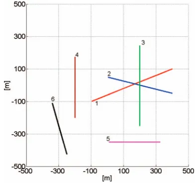
Fig. 1. Linear scenario used for performance evaluation. Six targets move inertially. Individual starting points of each target correspond to denoted target ID number. Targets 1 - 3 are present for all time steps.
Target 4 is present between time step 15 and 90. Targets 5 and 6 are present between time step 30 and 75.
face). In this paper we randomly pick a dimension to be divided for the selected box-particle. Next, rescale the weights byηkto get a new particle set{[xi], ηk/Nk+1}Ni=k+11.
The box-PHD filter is summarized as algorithm 1.
VI. NUMERICAL STUDIES
This section gives numerical studies for the proposed box-PHD filter algorithm. For comparison with traditional particle filter techniques we use a point particle SMC-PHD filter. As a performance measure the OSPA metric [21] is used for performance measure, together with the criteria for measuring the inclusion of the true state and the volume of the posterior pdf. The later two were introduced in [20, 30]. Both filters have been implemented in C+ + in a similar way. In addition the Boost Interval Arithmetic Library [31] was used to handle interval datatypes.
A. Testing Scenario
We analyze the behavior of both filters in a demanding linear scenario. Herein six inertial moved targets are placed in an areaA=[−500,500] m×[−500,500] m. The unit is assumed to be meters. The state space is S ⊂R4, where the first two components correspond to the xandycoordinates and the third and fourth correspond to their velocities. The measurement space consists of [x] and [y] measurements, soZ⊂IR2. New measurements occur for the sake of simplicity every second. The measurement noise is white Gaussian noise with a standard deviation σx =σy =15 m. The probability of detection is set equal
for all states topD
k([x])=0.95. Target placement and
measurements is estimated following a Poisson distribution with the mean value|A| ·ρA.
Algorithm 1The box-PHD filter In:{([xi], wi)}Ni=k1,Zk,Zk−1
Out:{([xi], wi)} Nk+1
i=1 ,{[ˆyj],Pˆj}
1) Predict target intensity
• ForI=1, . . . , Nkapply (50) to get˜xi.
• SampleNk,newmany new particles according toZk−1
• Weights for new particles arewi(24)
2) Compute correction term
• λk|k−1([zj]), according to (29)
3) Update target intensity
• For every particle ([˜xi], wi), withI=1, . . . , Nk+Nk,new
set the new weight according to (35). 4) Compute target states
• Compute the setJ(40)
• For allj∈J:
[ˆyj]=W1j Ni=k1wj,i[˜xi] (42)
5) Compute covariance matrices
• For allj∈J computePjaccording to (43)
6) Contract boxes
• [ˆxi]=[hCP]([˜xi],[z]) (46)
7) Resample
• Use a resampling strategy with subdivision of boxes to get
{([xi], wi)} Nk+1 i=1
p(nc)=
1 nc!
(A·ρA)ncexp(−|A| ·ρA), (49)
with|A|denoting the volume of an observed area andρAa
parameter describing the clutter rate. For this scenario we usedρA=4·10−6. Clutter measurements are generated
by an independent and identically distributed (IID) process.
To initialize the particle cloud at time step
tk=0, N0 ∈N+particles are distributed uniformly across the state spaceS, e.g.N0=1000. The weights are set to wj=1/N0.
Assuming a constant velocity model in two dimensions the prediction of the persistent particles can be modeled by
[˜xi]=
⎛ ⎜ ⎜ ⎜ ⎝
1 0 t 0
0 1 0 t
0 0 1 0
0 0 0 1
⎞ ⎟ ⎟ ⎟
⎠[xi]+[ν], (50)
witht =tk−tk−1andνa 3σ interval of some white process noise, defined by a covariance matrix. Hidden in (50) are inclusion functions for the individual
dimension of the state space. A close look reveals that every variable only appears once (for each dimension) and that all operations are continuous, so these natural
inclusion functions are minimal and the propagated boxes have minimal size. This fact holds for constant velocity models with arbitrary dimensions.
B. Performance Measures
Let us defined(c)(x,y) :=min(c, d(x,y)) as the distance betweenx,ycut off atc >0, andπlthe set of
permutations on{1,2, . . . , l}for anyl∈N= {1,2, . . .}. For 1≤p ≤ ∞, c >0, and arbitrary finite subsets X= {x1, . . . ,xm}andY= {y1, . . . ,yn}ofS, with m, n∈N0, the OSPA metric [21] is defined as
¯
dp(c)(X,Y)
:=
1 n
min
π∈n
m
i=1
d(c)(xi,yπ(i))p
+cp(n−m)
1
p
.
(51)
For the OSPA metric (51) we use directly the state
estimates if using the SMC-PHD filter. To apply the OSPA metric to the box-PHD filter we use the point state
estimatesˆyj gained in (41) of the proposed algorithm.
Alternatively, one can use the center points of the box states mid([ˆyj]), which have the same values asˆyj.
The inclusion valueρmeasures whether the state vector is contained in the support of the posterior pdf, or in the case of the PHD filter, the posterior intensity. Given the ground truth for all targetsy∗l, withlan index over the true number of targets, the inclusion for the SMC-PHD filter can be computed by evaluating
ρlSMC=
1 ∃j : (ˆyj−ˆy∗l)P−
1
j (ˆyj−ˆy∗l)T < κ
0 otherwise. (52)
The condition in (52) checks if the ground truth is
contained in the error ellipse defined by covariance matrix Pj. The termκdefines the size of the error ellipse, e.g. use
κ=11.8 for a 3σ–ellipse in two dimensions [32]. The inclusion for the box-PHD filter is much simpler to compute: check if the ground truthy∗l is contained in one of the state boxes [ˆyj]. If this is true the inclusion value is
one, otherwise zero. Thenρlfor the box-PHD filter is
given by
ρlbox=
1 fory∗
l ∈[ˆyj] and
0 otherwise. (53)
The volume criteria measures the spread of the particle distribution for a given state. To have a fair comparison between both filters we compute the volume for the SMC-PHD filter as
νjSMC=
6·Pj(1,1)+6·
Pj(2,2). (54)
The volume in (54) is the square root of the widths of a box containing the 3σ–ellipse of statej. Note that we only consider here the position information, since the entries of Pj have different units. For the box-PHD filter the volume
is computed as the square root of the widths of the box states, giving
νjbox=|[ˆyi](1)| + |[ˆyi](2)|. (55)
C. Simulations
1)Accuracy Test: In the first simulation we
Fig. 2. Visualization of proposed box-PHD filter. Green solid lines are true target trajectories. Blue solid boxes correspond to projection of estimated box states into 2D. Box-particles are visualized as dashed
[image:9.612.317.536.204.340.2]black boxes, while red dotted boxes are measurements.
Fig. 3. Mean OSPA values for 1000 Monte Carlo trials on linear scenario for both filters.
[image:9.612.68.284.264.394.2]the linear scenario described earlier. A visualization of the box-PHD filter for the linear scenario can be seen in Fig. 2. Fig. 3 shows the mean OSPA values achieved with both filters on the given scenario. We can observe that the OSPA values are in general very low. This means that the SMC-PHD filter and the box-PHD filter behave very well in this scenario. However, we can also observe that the box-PHD filter has a little higher values than the
SMC-PHD filter. The authors of [20] already noticed that point estimates gained from box-particles can have a slight bias. Therefore they introduced two new measurement criteria – inclusion and volume. The mean results for 1000 Monte Carlo trials and all targets are shown in Figs. 4 and 5, respectively. It can be easily seen that the inclusion and volume values react to target appearance and target disappearance. In general we can say that the box-PHD filter has a higher volume then the SMC-PHD filter. This can be seen as a drawback of the box-particle technique. However, a closer look at the inclusion values reveals that the higher volume leads to better values for the inclusion criteria. So we can state that the SMC-PHD filter converges quickly to the solution and therefore it can happen sometimes that the true target state is not in the support of any covariance matrixPj. From an engineering
Fig. 4. Mean inclusion values for 1000 Monte Carlo trials and all targets on linear scenario without biased measurements for both filters.
Fig. 5. Mean volume values for 1000 Monte Carlo trials and all targets on linear scenario without biased measurements for both filters.
Fig. 6. Mean estimated number of states for 1000 Monte Carlo trials on linear scenario.
[image:9.612.316.537.372.505.2]TABLE I
Mean Runtimes for Processing One Time Step
Processing time (ms) Speedup
SMC-PHD filter 10.3428 1.0
Box-PHD filter 0.95167 10.9
[image:10.612.65.307.60.106.2]Note:Values computed over 1000 Monte Carlo trials and for all time steps of the linear scenario.
[image:10.612.80.294.143.271.2]Fig. 7. Mean OSPA values for varying number of box-particles over time.
Fig. 8. Mean inclusion values for 1000 Monte Carlo trials and all targets on linear scenario with biased measurements for both filters.
published in [30]. Nevertheless, Fig. 7 shows mean OSPA values for 1000 Monte Carlo trials in the above scenario, where the number of box-particles used is varied. It can be seen that as few as 10 box-particles are needed in order to reach acceptable OSPA values. Worth mentioning is also that the maximum accuracy is already achieved by 50 box-particles for this scenario.
2)Strong Bias: In the next simulation we investigate the behavior of both filters when the sensor measurements have a strong bias, i.e., the bias is bigger than the white process noise of the sensor. The examples are similar to those considered in [33] and in [30]. The linear scenario is used again and we added to every measurement a bias of 30[m] for thexmeasurement and a bias of 10 for they measurement. The volume of both filters does not change, which can be seen in Fig. 9. The inclusion criteria on the other hand change dramatically for the SMC-PHD filter; the value drops to values around 0.5[m], c.f. Fig. 8. This means that approximately 50% of the time the true target state is not within the posterior intensity of the filter. This
Fig. 9. Mean volume values for 1000 Monte Carlo trials and all targets on linear scenario with biased measurements for both filters.
indicates filter divergence, which is considered a
catastrophic event in target tracking. The box-PHD filter, on the other hand, reaches values similar to the first simulation without bias. These results lead to the conclusion that the box-PHD filter outperforms the point SMC-PHD filter in scenarios with strongly biased measurements.
VII. CONCLUSION
In this paper we presented a novel technique for nonlinear multitarget tracking with a box-particle based filter, called the box-PHD filter. The theoretical backbone of this is the random finite set theory, which can be used to derive the general intensity filter equations. For the implementation, however, methods from interval analysis are used additionally to get a box-particle representation of the PHD filter. This representation allows a decrement of the number of particles needed. In our simulations we could reduce the number of particles by a factor of approximately thirty and reduce the computation time by a factor of approximately eleven. On the other hand, the accuracy of the filter was not remarkably reduced. Especially in the presence of strong bias we show that the box-PHD filter can outperform the SMC-PHD filter with point particles.
APPENDIX. CONTRACTION EXAMPLE
Assume the following scenario: a sensor measures azimuthαand rangerin a local sensor coordinate system. The objective is to track a target in a global Cartesian coordinate system with these measurements. A measurement is thenz=(α, r)T, while the state is
represented byx=(x, y)T. The point measurement
function is defined as
z=h(x)=
⎛ ⎜ ⎜ ⎝
arctan
y−y0 x−x0
(x−x0)2+(y−y0)2
⎞ ⎟ ⎟ ⎠
Constraint 1
Constraint 2 ,
(56) where (x0, y0)T is the sensor position in a global
[image:10.612.78.294.313.443.2]Fig. 10. Contraction example. Box [x] is contracted by measurement box [z]. Result is green box [x].
measurements [z]=[α]×[r] and box states [x]=[x]×[y], a contractor [hCP] ([x]|[z]) based on
constraint propagation [23] is given by the following algorithm:
0) Input: [x]=[x]×[y],[z]=[α]×[r] Output: [x]=[x]×[y]
1) for Constraint 1 do:
[x] :=[x]∩[x0]+
[y]−[y0]
[tan]([α]) (57)
[y] :=[y]∩[y0]+([x]−[x0])[tan]([α]) (58)
[α] :=[α]∩[arctan]
[y]−[y0]
[x]−[x0]
(59)
2) for Constraint 2 do:
[x] :=[x]∩[x0]+
[r]2−([y]−[y
0])2 (60)
[y] :=[y]∩[y0]+
[r]2−([x]−[x
0])2 (61)
[r] :=[r]∩([x]−[x0])2−([y]−[y0])2 (62)
3) if the boxes [x] and [z] are changed return to step 1.
The box [x0]×[y0] represents the sensor position as a singleton. In practice we found it useful to stop this iteration after a finite number of loops, e.g. three, without any lack of performance. The quotient of the contracted box volume and the original box volume is used to calculate the likelihood. Fig. 10 visualizes the idea.
REFERENCES
[1] Bar-Shalom, Y., and Fortmann, T.
Tracking and Data Association. San Diego, CA: Academic, 1988.
[2] Fortmann, T., Bar-Shalom, Y., and Scheffe, M.
Sonar tracking of multiple targets using joint probabilistic data association.
IEEE Journal of Oceanic Engineering,OE-8(1983), 173–184.
[3] Reid, D. B.
An algorithm for tracking multiple targets. IEEE Transsactions on Automatic Control,AC-24, 6 (1979), 843–854.
[4] Mahler, R.
Multitarget Bayes filtering via first-order multitarget moments.
IEEE Transactions on Aerospace and Electronic Systems,39, 4 (2003), 1152–1178.
[5] Panta, K., Vo, B.-N., Singh, S., and Doucet, A.
Probability hypothesis density filter versus miltiple hypothesis tracking.
Proceedings of SPIE, Vol. 5429, 2004, pp. 284–295. [6] Juang, R., and Burlina, P.
Comparative performance evaluation of GM-PHD filter in clutter.
InProceedings of the 12th International Conference on Information Fusion (FUSION ‘09), July 2009. [7] Bar-Shalom, Y., Fortmann, and Scheffe, M.
Joint probabilistic data association for multiple targets in clutter.
InConference on Information Sciences and Systems, 1980. [8] Sidenbladh, H.
Multi-target particle filtering for probability hypothesis density.
InInternational Conference on Information Fusion, Cairns, Australia, 2003, pp. 800–806.
[9] Zajic, T., and Mahler, R.
A particle-systems implementation of the PHD multi-target tracking filter.
Proceedings of SPIE, Vol. 5096,Signal Processing, Sensor Fusion Target Recognition XII, 2003, pp. 291–299. [10] Vo, B.-N., Singh, S., and Doucet, A.
Sequential Monte Carlo methods for multi-target filtering with random finite sets.
IEEE Transactions on Aerospace and Electronic Systems,41, 4, (2005), 1224–1245.
[11] Vo, B.-T., and Ma, W.-K.
The Gaussian mixture probability hypothesis density filter. IEEE Transactions on Signal Processing,55, 11 (2006), 4091–4104.
[12] Ristic, B., Clark, D., Vo, B.-N., and Vo, B.-T.
Adaptive target birth intensity for PHD and CPHD filters. IEEE Transactions on Aerospace and Electronic Systems,48, 2 (Apr. 2012), 1656–1668.
[13] Milanese, M., and Vicino, A.
Optimal estimation theory for dynamic systems with set membership uncertainty: An overview.
Automatica,27, 6 (1991), 997–1009. [14] Combettes, P.
Foundations of set theoretic estimation. Proceedings of the IEEE,81, 2 (1993), 182–208. [15] Kruse, R., Schwecke, E., and Heinsohn, J.
Uncertainty and Vagueness in Knowledge Based Systems. New York: Springer-Verlag, 1991.
[16] Smets, P.
Imperfect information: Imprecision and uncertainty. In A. Motto et al. (Eds.),
Uncertainty Management in Information Systems. Boston: KluwerAcademic Publishers, 1997, pp. 225–254. [17] Anderson, B. D. O., and Moore, J. B.
Optimal Filtering. Upper Saddle River, NJ: Prentice-Hall, 1979.
[18] Abdallah, F., Gning, A., and Bonnifait, P.
Box particle filtering for nonlinear state estimation using interval analysis.
Automatica,44(2008), 807–815. [19] Gning, A., Mihaylova, L., and Abdallah, F.
InProceedings of the 13th International Conference on Information Fusion, Edinburgh, UK, July 2010. [20] Gning, A., Ristic, B., and Mihaylova, L.
A box particle filter for stochastic set-theoretic measurements with association uncertainty.
InProceedings of the 14th International Conference on Information Fusion, Chicago, IL, July 2011.
[21] Schumacher, D., Vo, B.-T., and Vo, B.-N.
A consistent metric for performance evaluation of multi-object filters.
IEEE Transactions on Signal Processing,56, 8 (2008), 3447–3457.
[22] Mahler, R.
Multitarget Bayes filtering via first-order multitargets moments.
IEEE Transactions on Aerospace and Electronic Systems,39, 4 (2003), 1152–1178.
[23] Jaulin, L., Kieffer, M., Didrit, O., and Walter, E. Applied Interval Analysis. New York: Springer, 2001. [24] Ristic, B., Clark, D., and Vo, B.-N.
Improved SMC implementation of the PHD filter. InProceedings of the 13th International Conference on Information Fusion, Edinburgh, UK, July 2010. [25] Vo, B.-T., Vo, B.-N., and Cantoni, A.
The cardinality balanced multi-target multi-Bernoulli filter and its implementations.
IEEE Transactions on Signal Processing,57, 2 (2009), 409–423.
[26] Erdinc, O., Willett, P., and Bar-Shalom, Y.
Probability hypothesis density filter for multitarget multisensor tracking.
InProceedings of the 8th International Conference on Information Fusion(FUSION), Philadelphia, PA, July 2005.
[27] Erdinc, O., Willett, P., and Bar-Shalom, Y.
The bin-occupancy filter and its connection to the PHD filters. IEEE Transactions on Signal Processing,57, 11 (2009), 4232–4246.
[28] Crisan, D., and Doucet, A.
A survey of convergence results on particle filtering methods for practinioners.
IEEE Transactions on Signal Processing,50, 3 (2002), 736–746.
[29] Mahler, R., and El-Fallah, A.
The random set approach to nontraditional measurements is rigorously Bayesian.
Proceedings of SPIE, Vol. 8392,Signal Processing, Sensor Fusion, and Target Recognition XXI, 2012, pp. 83 920D–83 920D–10. [Online]. Available:
http://dx.doi.org/10.1117/12.919824. [30] Gning, A., Ristic, B., and Mihaylova, L.
Bernoulli particle / box-particle filters for detection and tracking in the presence of triple measurement uncertainty. IEEE Transactions on Signal Processing,60, 5 (2012), 2138–2151.
[31] Boost interval arithmetic library. [Online]. Available: www.boost.org/doc/libs/1_53_0/libs/numeric/interval/doc/ interval.htm. Dec. 2006.
[32] Press, W., Flannery, B., Teukolsky, S., and Vetterling, W. Numerical Recipes in C: The Art of Scientific Computing (2nd ed.). New York: Cambrige University Press, 1992.
[33] Ristic, B., Clark, D. E., and Gordon, N.
Calibration of multi-target tracking algorithms using non-cooperative targets.
IEEE Journal of Selected Topics in Signal Processing,7, 3 (June 2013), 390–398.
Marek Schikorareceived a BS (Vordiplom, 2006) and the MS (Diplom, 2008) in computer science from the University of Bonn, Germany. He is a Ph.D. student at the Computer Vision Group at the Technical University of Munich, Germany.
Since 2009 he has been a research scientist in the Sensor Data and Information Fusion Department at Fraunhofer FKIE, Germany, where he is leading a research team with a focus on aerial vision. His research is focused on sensor fusion, multitarget tracking and related computer vision topics, like image segmentation, object detection, and classification.
Amadou Gningreceived his PhD degree in the area of “technologies of information and systems” at the Universit´e de Technologie de Compi`egne, France in 2006.
Lyudmila Mihaylova(SM’08) is an Associate Professor with the University of Sheffield, Department of Automatic Control and Systems Engineering, United Kingdom. From 2006 to 2013 she was with the University of Lancaster, United Kingdom. Her interests are in the areas of nonlinear filtering, sequential Monte Carlo Methods, statistical signal processing, and sensor data fusion. Her work involves the development of novel Bayesian techniques, e.g. for high dimensional problems (including for vehicular traffic flow estimation and for image processing), localisation and positioning in sensor networks.
Dr. Mihaylova has published book chapters and numerous journal and conference papers in the areas of her research interests. She is the Editor-in-Chief of theOpen Transportation Journaland an Associate Editor of theIEEE Transactions on Aerospace and Electronic SystemsandElsevier Signal Processing Journal. She is a member of the International Society of Information Fusion (ISIF). She has given a number of invited tutorials including for the COST-NEARCTIS workshop and is involved in the
organization of international conferences/ workshops. Her research is funded by grants from the EPSRC, EU, MOD, and industry.
Daniel Cremersreceived the MS (diploma) degree in theoretical physics from the University of Heidelberg, Germany in 1997, and the PhD degree in computer science from the University of Mannheim, Germany, in 2002.
He spent two years as a postdoctoral researcher at the University of California, Los Angeles, and one year as a permanent researcher at Siemens Corporate Research, Princeton, NJ. From 2005 to 2009, he headed the Computer Vision Group at the University of Bonn, Germany. Since 2009, he has been a full professor at Technical University of Munich.
Dr. Cremers has received several awards, in particular, the Best Paper of the Year Award 2003 by the Pattern Recognition Society, the Olympus Award 2004, and the 2005 UCLA Chancellor’s Award.
Wolfgang Koch(F’10) PD Dr. habil, studied physics and mathematics at RWTH Aachen, Germany.
He is head of the Dept. of Sensor Data and Information Fusion at Fraunhofer FKIE, a research institute active in defence and security.
Dr. Koch has published several handbook chapters and numerous