Non-intrusive load disaggregation using graph signal processing

Non-Intrusive Load Disaggregation using Graph

Signal Processing

Kanghang He, Lina Stankovic, Jing Liao, and Vladimir Stankovic

Abstract—With the large-scale roll-out of smart metering worldwide, there is a growing need to account for the individual contribution of appliances to the load demand. In this paper, we design a Graph signal processing (GSP)-based approach for non-intrusive appliance load monitoring (NILM), i.e., disaggregation of total energy consumption down to individual appliances used. Leveraging piecewise smoothness of the power load signal, two GSP-based NILM approaches are proposed. The first approach, based on total graph variation minimization, searches for a smooth graph signal under known label constraints. The sec-ond approach uses the total graph variation minimizer as a starting point for further refinement via simulated annealing. The proposed GSP-based NILM approach aims to address the large training overhead and associated complexity of conven-tional graph-based methods through a novel event-based graph approach. Simulation results using two datasets of real house measurements demonstrate the competitive performance of the GSP-based approaches with respect to traditionally used Hidden Markov Model-based and Decision Tree-based approaches.

Index Terms—energy disaggregation, graph signal processing, energy feedback, smart metering

I. INTRODUCTION

Appliance-level load demand information significantly en-riches customer energy feedback and improves demand man-agement measures via, for example, appliance load shifting [2]. While appliance-level energy monitors can yield accurate measurements, an alternative approach is preferred that is non-intrusive and accommodates the ever increasing number of appliances in a household, minimizing maintenance and instal-lation costs due to sensor lifetime and networking/security is-sues. Hence, non-intrusive appliance load monitoring (NILM), i.e., disaggregation of the household aggregate load down to individual appliances, based purely on analytical tools operat-ing only on aggregate load data, has been gainoperat-ing popularity, especially with ongoing smart meter roll-outs worldwide. The business case for NILM is presented in [3], showing that resulting energy savings significantly surpass the costs of NILM technologies. NILM can support retrofit appliance advice, demand response measures, smart home automation [4], and is an enabler in decision making for home-owners, utilities, appliance manufacturers and policy makers.

Though NILM appeared in the 1980’s [5], there has been a recent explosion in the NILM literature to tackle its practical

The authors are with the Dept. Electronic and Electrical Engineering, University of Strathclyde, Glasgow, G1 1XW, UK. Email: {kanghang.he, lina.stankovic, jing.liao, vladimir.stankovic}@strath.ac.uk. Part of this work was presented atIEEE Symp. Series Comput. Intelligence (SSCI-2014)[1].

This work was supported in part by the UK Engineering and Physical Sci-ences Research Council (EPSRC) project REFIT EP/K002368.The data used in this paper can be accessed at http://dx.doi.org/10.15129/31da3ece-f902-4e95-a093-e0a9536983c4(REFIT) andhttp://redd.csail.mit.edu/(REDD).

challenges. NILM methods can be divided into two groups: steady-state and transient-state methods. Steady-state NILM methods rely on features extracted under steady-state operation of appliances, e.g., changes in steady-state active power [6], [7], [8], [9], reactive power [5], voltage and current wave-form [10], [11], steady-state current harmonics and total har-monic distortion [12], [13], or voltage-current trajectory [14]. Transient-state NILM methods identify appliances based on their transient signatures, including transient power [15], high frequency voltage noise [16], [17], harmonics of the transients [18], [19], [20], duration and shape of power/voltage/current transient waveform [21], [22]. Transient-state approaches provide more distinguishable features than steady-state ap-proaches and hence, in general, lead to higher disaggregation accuracy. Transient methods require sampling rates in the order of kHz or MHz [23], unlike steady-state methods, which are more sensitive to power level fluctuations and at low sampling rates, require longer monitoring time to capture all operation cycles [24]. For a more detailed review of NILM, see review papers [21], [23].

The proposed low-rate NILM approach in this paper is motivated by the increasing availability of low-rate data from electricity smart meters that are being deployed at large scale, with an increasing penetration rate, in Europe, Australia and the USA. For example, in the UK [25] and The Netherlands [26] every household will have access to 10-second active power readings. In the USA and Australia, smart meters providing readings at rates in the order of seconds and minutes, are massively deployed. Thus, NILM outputs can be accessible to the average household, without additional metering or monitoring hardware. This has prompted a recent trend in NILM literature tackling the NILM problem at low sampling rates, for example, [6], [7], [8], [27], [28], [29]. However, at low sampling rates, only steady-state features can be extracted reliably. Due to the similarity of steady-state load signatures among many domestic appliances, the NILM problem is particularly challenging.

for disaggregation of active power loads sampled at 1min, using expert knowledge to build initial models for states of known appliances, requiring correctly setting a priori-values for each state for each appliance, which is in turn limited by or strongly dependent on the particular aggregate dataset on which NILM is being performed. The Hierarchical Dirichlet Process Hidden Semi-Markov Model factorial structure is used in [30], removing some limitations of the approach of [27], but at increased complexity. A sparse coding algorithm, that discriminately trains sparse coding dictionaries, is proposed in [31], to learn a probabilistic model for each appliance’s load demand over a typical week. The HMM-based method of lower complexity, proposed in [32], reduces the execution time by 72.7 times, but still requires 94 minutes for disaggregating 11 appliances. The main drawback of state-based approaches is the need for expert knowledge to set a-priori values for each appliance state via long periods of training and their high computational complexity, which makes them unsuitable for real-time applications [33].

Event-based NILM approaches have thus emerged [34], which are based on detecting events, usually via edge detec-tion, when the load signal undergoes a statistically signifi-cant change indicating appliance use. After event detection, features (e.g., active power signature, increasing/falling edge [8], duration [35], uncorrelated power spectral components [6]) are extracted to classify the events into pre-defined cat-egories, each corresponding to a known appliance. Different classification tools have been used, including support vector machines (SVM), e.g., in [36], neural networks, e.g., in [37], nonnegative tensor factorization [9], k-means [35] and decision trees [8]. Challenges encountered by event detection tools include large measurement noise, including large variance of active power readings for common household appliances, and similarity among active power steady-state signatures of different appliances.

This paper presents a different approach, developing agraph signal processing (GSP) method for steady-state NILM to address the large training overhead and associated complexity of conventional graph-based methods through a novel event-based graph approach. GSP [38] is an emerging field that relies on expressing the piecewise smoothness of a signal through a graph. In [39], a GSP-based data classifier is proposed that searches for a smooth graph signal under known label con-straints, and is applied to image and document datasets. The approach is based on the regularization of graph signals, using the fact that if a signal is piecewise smooth, then the total graph variation is generally small. Inspired by [38] and [39], in this paper, we propose a GSP-based approach for NILM by posing the load disaggregation problem as a single-channel blind source separation problem [31] to perform low-complexity classification of active power measurements. We treat active power measurements as a signal, indexed by the nodes of an undirected graph where each vertex corresponds to the signal sample, and the weights of the edges connecting the vertices reflect the degree of similarity between the nodes, i.e., the weights of the edges enable ‘grouping’ on/off events from the same appliance. Then, we define an optimization problem that contains the regularization term of the total graph variation,

that is, we apply regularization on the constructed graph signal to find the signal with minimum variation. However, unlike the approach in [39], which solves for a smooth graph signal using initially known labels as prior, to avoid over-smoothing, we use the total graph variation minimizer as a starting point to minimise the difference between the total measured power and the sum of the disaggregated loads, deviating from traditional NILM approaches (see [23], [9] and references therein).

The rest of the paper is organized as follows. Sec. II provides a short background on GSP. Sec. III describes the proposed GSP-based NILM algorithms, followed by results in Sec. IV. The last section concludes the paper and highlights future work.

II. GRAPH SIGNAL PROCESSING(GSP)

In this section, we describe some basic concepts of GSP. All matrices are denoted by upper-case bold letters, such as X.XT _andX#_{are the transpose and pseudo-inverse matrices}

of X, respectively. An element in thei-th row and j-column of matrixXis denoted byXi,j. Vectors are denoted by

lower-case bold letters, such asx, with thei-th elementxi, andxi:j

denotes a sub-vector [xi, xi+1, . . . , xj]T, for i < j. A set is

denoted using calligraphic bold-letters, such asM, where|M| denotes its cardinality.

GSP is a novel signal processing concept [38], [40] that ef-fectively captures correlation among data samples in time and space by embedding the structure of signals onto a graph [40] leading to a powerful, scalable and flexible approach suitable for many data mining and signal processing problems, ranging from image denoising and data compression, to classification, biomedical, and environmental data processing (see [38], [39], [40], [41] and references therein). GSP is particularly suitable for data classification when training periods are short and insufficient to build appropriate class models [39].

In GSP, a dataset x is represented by a discrete signal s indexed by the nodes of a graph G = (V,A), where V is the set of nodes andAis a weighted adjacency matrix of the graph. Each element xi ∈ x corresponds to a node vi ∈ V.

The weight of the edge between nodes vi andvj reflects the

similarity between xi and xj and is usually defined using a

Gaussian kernel weighting function, which is one of the most used kernels in machine learning for expressing similarity between dataset elements:

Ai,j= exp n

−(xi−xj)2

σ2

o

, (1)

whereσis a scaling factor. Then,s, often referred to asgraph signal, is defined as a mapping fromV to a set of complex numbers. For example, scan be a set of classification labels, wheresi is set to the label of the class thatxi belongs to.

We define a graph signal’s total Lipschitz smoothness [38], [42] with respect to the intrinsic structure of the underlying graphG as:

1 2

N X

i=1 N X

j=1

Ai,j si−sj 2

. (2)

It can be shown that (2) is equal tosT_{Ls[38], where anN×N}

Laplacian matrixL is defined as

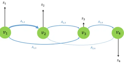
Fig. 1. A GSP example with four nodes.

which is a real symmetric matrix and can be seen as a differ-ence operator for the graph signals[38]. In (3),Dis anN×N

diagonal matrix where fork= 1, . . . , N,Dk,k=P N j=1Aj,k.

Eigenvalues ofLcarry the notion of frequency spectrum ofs, where values of eigenvectors associated with low eigenvalues (low frequency) change less rapidly [38] across the nodes, which can be used to design graph signal filters.

Fig. 1 shows an example with four nodes. The thickness of the graph edges reflect the correction between the nodes and vertical lines correspond to the graph signal values. If the graph signalsis piecewise smooth with respect to the graphG, then (2) will be generally small, which can be used as a prior for regularization. Indeed, in classification [39], the elements that are strongly correlated will be connected via high-weight edges and associated with the same classification labels si

makingsvarying smoothly across the connected nodes in the graph.

III. METHODOLOGY

A. Problem Formulation

Let M be the set of all known appliances in the house and p(ti) the measured aggregate active power of the entire

house measured at time ti. Without loss of generality, in the

following, we denote p(ti)asp(ti) =pi≥0. Letpmj ≥0 be

the power load of appliancem∈ Mat time instancetj.

Let ∆pi=pi+1−pi and∆pmi =p m i+1−p

m i . Then,

pi= |M| X

m=1

pm_i +ni, (4)

where,niis the measurement noise that also includes baseload

and all unknown appliances running. The disaggregation task is, for i= 1, . . . , N andm∈ M, givenpi, to estimatepmi . B. GSP-based Disaggregation

To tackle the disaggregation problem using the GSP frame-work, we construct a graph G = (V,A), where each vertex

vi ∈ V is associated to one sample ∆pi, i = 1, . . . , N.

For training, we assume availability of pi and pmi , for i =

1, . . . , n < N, for allm∈ M. Then, the task is to estimate

pm_i , for n < i≤N.

LetT hrm≥0be a power threshold for appliancemwhich

is set during training (see Sec. IV) in such a way that if

the magnitude of the appliance active power change is larger than the power threshold, then we assume that the appliance changed its operation state (e.g., switched on/off). Then, we define anN-length graph signalsm _{for Appliancemas:}

smi =   

 

+1, for |∆pm_i | ≥T hrmandi≤n

−1, for |∆pm

i |< T hrmandi≤n

0, for i > n.

(5)

Note thatsm_i can be seen as a set of classification labels, where during training (i≤n)sm_i is set to +1 (elementibelongs to Appliance m class) or -1 (element i does not belong to the class), depending whether the appliance changed state or not. Since for the testing dataset (i > n) we do not know if the appliance was running, we set corresponding values ofsm

i to

0.

We can now calculate adjacency matrixAaccording to (1), where xi = ∆pi. The graph smoothness can be calculated

using (2). Letri=

h

∆p1_i,∆p2_i,· · ·,∆p|M|_i

i

and let the difference be-tween the actual aggregate power and the sum of disaggregated appliance powers be:

f(ri) = ∆pi−

P|M| m=1∆p

m i

2

2. (6)

We pose the disaggregation optimization problem as min-imization ofPN

i=n+1f(ri) using piecewise smoothness as a

prior by introducing (2) as a regularization term, i.e.,

min

[rn+1,···,rN]

N X

i=n+1

f(ri) +ω X

m∈M s

mT Lsm

2

2 . (7)

Note that (7) defines an optimal solution as the smoothest solution that minimizes (6), whereωis a parameter that trades off smoothness and the minimization (6).

(7) is a hard optimization problem especially since |M| andN−ncan be large. Thus, we propose two approximate solutions, one minimizing only the second term in (7), and the other minimizing both terms iteratively.

C. Solution 1: Total Graph Variation Classifier

If we assume, as in [39], that the true classification labels form a low-frequency graph signalsm, then for each Appli-ancem, an individual classifier can be defined that minimizes

s

mT_Lsm 2

2

, i.e., one that finds the smoothest signal. We call this classifier, the total graph variation classifier. The intuition behind it is that the labeled training samples for

i≤nthat are close in value to the unknown samples,j > n, will have large edge weights Ai,j, and so a smooth

graph-signal prior will ensure that the testing samples have similar classification as these training samples.

Since sm

1:n is known, determined during training, we can

simplify the smoothness term as [41]:

smTLsm=sm_1:nTL1:n,1:nsm1:n+

sm_1:nTL1:n,n+1:Nsmn+1:N+

sm_n+1:NT Ln+1:N,1:nsm1:n+

sm_n+1:NT Ln+1:N,n+1:Nsmn+1:N.

Since matrix A is symmetric, D is diagonal and L is diagonally symmetric, it follows that:

sm_1:nTL1:n,n+1:Nsmn+1:N =s mT

n+1:NLn+1:N,1:nsm1:n. (9)

Using (9), and sincesm1:nis constant, the first term does not

affect minimization, we minimize (8) as:

arg min s

mT Lsm

2

2

= arg min{2sm_n+1:NT Ln+1:N,1:nsm1:n+

sm_n+1:NT Ln+1:N,n+1:Nsmn+1:N}.

(10)

This is an unconstrained quadratic programming problem with a closed form solution [41], [43]:

sm∗=L#_n+1:N,n+1:N−smT

1:n

LT_1:n,n+1:N. (11)

Once sm∗ is determined, for i > n, if sm_i ∗ > Ts, then,

Appliance m changed state,∆pm_i ∗ is set to the mean of pm_i

which is calculated through the training process; otherwise, Appliance mdid not change its state, and ∆pm∗

i = 0.

In contrast to [39], where the threshold Ts is set to zero,

we set our classification threshold Ts =0.5, which imposes

that only samples that are highly correlated with the training samples will be assigned to the same class. The value of 0.5 was found heuristically to yield the fewest false positives without increasing the number of false negatives.

We repeat minimisation of the smoothness term for all appliances m ∈ M, where after each appliance has been disaggregated, its contribution to the total load is removed by subtracting its mean from the aggregate. Note that the same nodes are used for all appliances, but matrix Achanges with updated ri∗, i=n+ 1,· · ·, N.

Fig. 2. An example of GSP-based disaggregtoin.

An example is given in Fig. 2. The top figure shows the generated graph nodes and connections between the nodes. Note that each node corresponds to one active power reading shown in the middle graph. The graph signal (shown on the bottom graph) contains classification labels for each power edge. During testing (i > n) all calculated values ofsmabove thresholdTs= 0.5will be classified to the Appliancemclass,

i.e., there was appliance state change or event.

The flow chart of the algorithm is shown in Fig. 3. The complexity of the approach depends on N −n since it is necessary to find the pseudo-inverse of an(N−n)×(N−n)

real-valued matrix, which can be done in O((N−n)3_{) time.}

Fig. 3. Flow chart for Solution1: Total Graph Variation Classifier.

D. Solution 2: GSP + Simulated Annealing Refinement

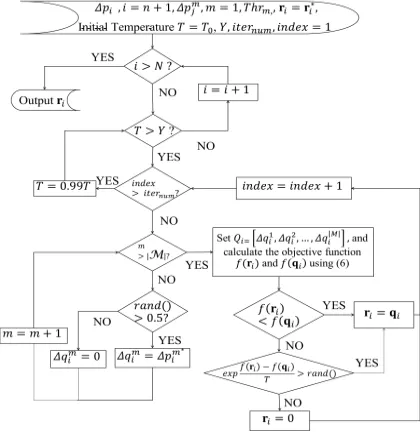
Fig. 4. Flow chart for Solution 2.r∗_i,i =n+ 1,· · ·, N is the solution found by Solution 1.

First, we apply Solution 1 based on (11), which is the starting point for the simulated annealing method [44] that will attempt to refine the result by minimising the first term of (7). We demonstrate in the next section that simulated annealing provides a solution identical or close to a greedy full-search method, which has exponential complexity in |M|.

The flow chart of Solution 2 is shown in Fig. 4. Note that the input is,r∗_i, i=n+ 1,· · · , N, which is a solution found by Solution 1. This solution is refined via iterative simulated annealing, whereiternumdenotes the number of iterations. In

each iteration, a candidate solutionqi is formed by randomly

setting appliances on/off. Step expnf(ri)−f(qi)

T o

> rand()

ensures that when the “temperature” T is high, the algorithm does not accept a worse solution, where rand()is a function that returns a random number in the interval (0,1). We heuristically demonstrate the convergence of the algorithm in the next section.

IV. EXPERIMENTALRESULTS ANDDISCUSSION

In this section, we present the following results: (1) Relative performance of using Simulated Annealing (SA) vs. Full Search, (2) Relative performance of Solution 1, SA only and Solution 2, (3) Comparison with state-of-the-art methods of [8] and [7], (4) Computational complexity.

We use the publicly available REDD dataset that contains load data from US houses [45], downsampled to 1min res-olution, and the REFIT dataset [4], one of the largest UK datasets that contains active power measurements, sampled at 8 sec resolution, and collected over a continuous period of 2 years from 20 UK homes. The REDD dataset contains clean data and a small number of unknown appliances. On the other hand, the REFIT dataset contains many unknown appliances and high variations in the baseload. For validation purposes, household appliances, for which timestamped individual power consumption is available via submetering, are treated as known appliances. They are: Dishwasher (DW), Refrigerator (REFR), Microwave (MW), Washer dryer (WD), Kitchen outlet (KO), Stove (ST), air-conditioning high (ACH) and low (ACL)

state, Electronics (EL), Washing machine (WM), Kettle (KE), Electric shower (ES), Electric heater (EH), Freezer (FRZ), Fridge-freezer (FFRZ). Baseload and Unknown appliances are abbreviated as BL and UN, respectively.

For training with the proposed methods, for each appliance, we used a period in the aggregate dataset when only that appliance is running (together with the BL). If a new appliance is introduced in the household, the training dataset is updated with that particular appliance’s signature, comprising samples representing a full run from on to off. No retraining needs to be performed for other appliances. At least 14 days worth of data is used for testing.

T hrm is always set to one half of the difference between

mean values of Appliancem’s consecutive states. For example, if a two-state appliance, on and off, T hrm would be half of

the power value in the on-state. The scaling factorσis picked during training in the area from the first non-zero value of the smoothness term to the inflection point, which was shown to provide the highest performance. For SA, temperature thresh-old Y = 0.01, T0 = 100|M| and iternum = 1000 which

trades off performance and complexity. For both proposed algorithms, we use windows of size 1000 samples, which ensures low complexity (see Subsection IV-D).

The evaluation metrics used are precision (PR), recall (RE) and F-Measure (FM) [46] defined as:

P R=T P/(T P +F P) (12)

RE =T P/(T P +F N) (13)

FM = 2∗(P R∗RE)/(P R+RE), (14)

where true positive (TP) is recorded when the detected ap-pliance was actually used, false positive (FP) is when the the detected appliance was not running, and false negative (FN) indicates that the appliance operation was not detected. Precision captures the correctness of detection - the higher the

P R, the fewer the FPs. On the other hand, high RE means a low number of FNs, which implies that a higher percentage of appliance state changes are detected correctly.FM balances P RandRE.

In addition, we use the average normalized error metric to measure the total energy difference between power estimated by the NILM algorithm and the actual power consumed, across all known appliances, which is defined as:

AN E=

PN

i=1p¯i−P N i=1pˆi

PN i=1p¯i

, (15)

wherepˆiis the power estimated by the NILM algorithm from

all disaggregated appliancesm ∈ M at time i and p¯i is the

actual power consumed by all known appliances at timei. This measure is useful, e.g., for appliance-itemized billing, when quantifying, across a fixed period of time, the error incurred by the NILM algorithm in estimating the total power consumed by individual appliances.

A. Full-Search vs Simulated Annealing

Fig. 5 shows an example of the convergence of the SA algorithm. It can be seen that the method converges after less than 300 iterations. Similar results are obtained for different datasets.

A full-search method can be used to minimize (6) off-line when|M| is small. Assuming only two-state appliances (i.e., ON/OFF), for each sample i, each appliance can either be switched on or off, or does not change state. Thus, with full-search, there are 3|M| possible combinations that should be inspected for each sample. Table I shows theFM value

com-parison between the full-search method and SA for two houses from the REDD dataset. One can see that the proposed sub-optimal SA approach finds a solution that is either identical to or very close to the full-search method.

B. SA, Solution 1 and Solution 2 Comparison

Fig. 5. Convergence of the simulated annealing method for House 2 from the REDD dataset.

TABLE I

SAVS.FULL-SEARCH(FS)FORREDD HOUSE(H) 2AND6.

REFR ST MW KO EL ACH ACL DW

FS H2 0.84 0.31 0.91 0.83 - - - 0.62 SA H2 0.84 0.30 0.91 0.83 - - - 0.62 FS H6 0.77 0.75 0.77 0.55 0.48 0.92 0.56 -SA H6 0.77 0.75 0.77 0.55 0.48 0.92 0.53

-Solution 1, lead to significantly worse FM performance for

some appliances than treating them jointly (Solution 2). When minimizing Equation (6), SA only uses known mean values ofpm

i and thus does not account for small fluctuations

in actual instantaneous pm_i . SA results in Table II are poor for Stove, since Stove (mean pm_i = 408W) is often confused with the low-power state of Dishwasher (mean pm_i =349W). Similarly, in Table III, Kitchen Outlet and Electronics have similar operating power states, hence they are often incorrectly labelled.

SA only does not outperform Solution 1, however the advantage of Solution 2 (integrating Solution 1 and SA) is consistent across all appliances and especially significant for appliances such as Electronics and AC.

TABLE II

THEFM RESULTS FORREDD HOUSE2.

Appliance REFR ST MW KO DW

Avg.Power [W] 171 408 1840 1056 1201 (349) Solution1 0.81 0.81 0.91 0.85 0.83

SA 0.84 0.30 0.91 0.83 0.62

Solution2 0.84 0.86 0.93 0.88 0.84

TABLE III

THEFM RESULTS FORREDD HOUSE6.

Appliance REFR ST MW KO EL ACH ACL

Avg.Power [W] 149 1724 1352 946 815 2376 357 Solution1 0.77 0.92 0.91 0.86 0.28 0.94 0.53 SA 0.77 0.75 0.77 0.55 0.48 0.92 0.56 Solution2 0.78 0.92 0.91 0.88 0.66 1.00 0.79

C. Comparison with state of the art

A comparison of performance of Solution 2 with the state-of-the-art NILM approaches, namely Decision Tree (DT) approach [8] and HMM-based approach [7] is shown in Tables IV, V, and VI for REDD Houses 1, 2, 6, respectively.

TABLE IV

COMPARISON BETWEEN THE PROPOSEDSOLUTION2 (P), HMMAND

DT-BASED METHODS FORREDD HOUSE1.

Appliance REFR MW DW KO WD FMp 0.88 0.70 0.57 0.39 0.89

FMHM M 0.97 0.50 0.13 0 0

FMDT 0.88 0.85 0.39 0.19 0.88

TABLE V

COMPARISON BETWEEN THE PROPOSEDSOLUTION2 (P)ANDHMMAND

DT-BASED METHODS FORREDD HOUSE2.

Appliance ST REFR KO MW DW FMp 0.86 0.84 0.88 0.93 0.84

FMHM M 0.21 0.90 0.68 0.47 0.04

FMDT 0.33 0.97 0.92 0.97 0.32

TABLE VI

COMPARISON BETWEEN THE PROPOSEDSOLUTION2 (P), HMMAND

DT-BASED METHODS FORREDD HOUSE6.

Appliance ST REFR KO MW AC EL FMp 0.92 0.77 0.88 0.91 0.88 0.66

FMHM M 0 0.88 0 0 0.12 0.03

FMDT 0.67 0.99 0 0 0.89 0

The proposed method was also tested using the noisy REFIT dataset [4]. The REFIT households were monitored remotely and uninterruptedly, while they were going about their usual domestic routines. Each house contains numerous appliances that were not monitored, including oven, lights, chargeable devices, small electronics, etc., which are considered unknown and contribute significantly towards noise. Tables VII and VIII show results for REFIT Houses 2 and 17, respectively. These two houses were selected as two houses which had relatively fewer unknown appliances compared to other houses in the dataset.

TABLE VII

COMPARISON BETWEEN THE PROPOSEDSOLUTION2 (P), HMMAND

DT-BASED METHODSREFIT HOUSE2.

Appliance FRZ WM DW TV MW KE FMp 0.77 0.55 0.62 0.49 0.95 0.88

FMHM M 0.49 0.26 0 0.06 0.01 0.01

FMDT 0.33 0.73 0.36 0 0.95 0.58

TABLE VIII

COMPARISON BETWEEN THE PROPOSEDSOLUTION2 (P), HMMAND

DT-BASED METHODS FORREFIT HOUSE17.

Appliance FRZ FFRZ KE MW WM FMp 0.64 0.76 0.96 0.81 0.76

FMHM M 0.32 0.19 0.01 0.22 0.01

FMDT 0.81 0.79 0.97 0.71 0.50

TABLE IX

REDD HOUSE1AND2. THE TOTAL DEMAND FOR TWO WEEKS WAS158

KWH AND77KWH FORHOUSES1AND2,RESPECTIVELY.

REFR MW ST KO DW WD BL UN

H1 14% 8% - 1% 7% 10% 22% 39%

H2 31% 8% 2% 1% 5% - 16% 37%

TABLE X

REFIT HOUSE2. TOTAL MONTHLY DEMAND WAS372KWH.

FFRZ WM DW TV MW KE ES BL UN

7% 4% 12% <1% <1% 6% 15% 18% 35%

TABLE XI

REFIT HOUSE17. TOTAL MONTHLY DEMAND WAS341KWH.

FRZ FFRZ KE MW WM EH ES BL UN

15% 7% 8% 2% 2% 11% 8% 21% 27%

With respect to disaggregation accuracy, theAN Emeasure given by (15), which measures the discrepancy between the true consumption and the disaggregated values, is, for REDD Houses 1 and 2, 7.33% and 6.91%, respectively, and for REFIT Houses 2 and 17, theAN Eis 8.97% and 9.24%, respectively. These results demonstrate that a very small percentage of the total load is wrongly disaggregated.

1) Discussion: As can be seen from Tables IV, V, and VI, the proposed method significantly outperforms the HMM-based approach for all appliances in the REDD dataset except the refrigerator. HMM usually performs well disaggregating the refrigerator due to continuous and sole operation (i.e., without any other appliances running) during the night and hence large data availability for learning and improving initial models [7], [8]. The poor performance for other appliances can be attributed to the short training period. The proposed method shows better or similar performance to the method of [8] expect for microwave in Houses 1 and 2, and refrigerator in most houses. These appliances have very small power fluctuations during operation, and hence the decision tree classifier based on the rising and falling power edge works especially well.

Tables VII and VIII show poor HMM results for the REFIT dataset due to the noise and many unknown appliances. The proposed solution is again better than or equal to the benchmark methods for most of the appliances except washing machine in House 2, where DT performs the best due to very distinctive high-state washing machine power edges.

The results for both REDD and REFIT dataset demonstrate that the proposed method provides more accurate disaggre-gation than the benchmark methods for most appliances. The difference is especially pronounced for the kitchen appliances,

namely Kettle, Microwave, and Stove. This is due to the fact that Stove and other kitchen appliances normally have a short operation time and relatively high power, thus machine-learning based approaches cannot generate probabilistic mod-els that accurately capture appliance operation. The HMM-based approach is sensitive to noise and suffers from a short training period. The DT-based method works well for appliances that have small fluctuations in load during their steady-state operation.

The results for multi-state appliances (dishwasher, washing machine) are generally worse for all tested algorithms. This is due to first, the fact that low-power operating states are often difficult to detect since they are ‘hidden’ in the baseload and noise. Second, since these appliances are on for a very longer period, many appliances are likely to run in parallel, adding to noise. Finally, multi-state appliances are not used frequently, thus it is more difficult to isolate good training periods.

On the other hand, cold appliances, refrigerator, freezer and fridge-freezer, are always on and have regular periodic signatures; thus the algorithms show good accuracy. However, due to higher level of noise from many unknown appliances, slightly worse results are obtained for the REFIT dataset with a higher false positive rate.

The TV in REFIT House 2 is hard to identify since it has relative low operating power and thus it is often hidden by noise and baseload. In addition, TV runs usually for a long period of time, and thus many appliances will run in parallel. Still, the proposed method is more successful than the benchmark methods, since it is less sensitive than HMM to the training dataset that does not have any instances of TV running alone and it is more successful in resolving the cases when multiple appliances run in parallel than DT. Electronics in REDD House 6 include different electronics equipment which produce complex power signatures that lead to worse results. The proposed algorithm again shows more robustness than the benchmark methods in this situation, since it is less sensitive to fluctuations in steady-state power signature during training and testing.

D. Computational complexity

The proposed algorithm was implemented in Matlab2015b and executed on an Intel(R) Core(TM) i5-3470 CPU @ 3.20GHz machine running Windows 7 64-bit. Table XII shows the computational time needed to disaggregate the refrigerator, which is periodically on, in the REDD House 1 for various testing set sizes N−n. The shaded row shows the accuracy when the testing dataset of size N−n is split into windows of 1000 samples each, and each window is independently processed, this way reducing the dimension of matrix L and hence lowering the complexity of calculation in (11). The bottom unshaded row shows the accuracy when the entire testing dataset is processed in one go - it also shows indirectly the effect of using only one ‘window’ of size 1000, 2000, 3000 etc. Similar FM values in all cases confirm that splitting the

testing dataset in smaller manageable ‘windows’ significantly reduces execution time without a loss in performance. The table also shows that the proposed method performs well with a small training overhead, i.e., increasing the number of samples in the testing dataset does not improve performance. Note that a window size of less than 1000 would not capture a full run of appliances with long operation period, such as washing machines or AC.

TABLE XII

COMPUTATION TIME OF THE PROPOSEDSOLUTION2FORREFRINREDD HOUSE1. THE SHADED ROWS SHOW RESULTS OBTAINED USING SMALL WINDOWS OF1000-SAMPLES EACH. THE BOTTOM ROWS SHOW RESULTS

WHERE THE TRAINING DATASET IS NOT SPLIT.

N−n 1000 2000 3000 4000 5000 6000 7000 Time [s] 1.33 3.22 3.86 4.41 4.99 5.52 6.01 FM 0.89 0.89 0.90 0.90 0.90 0.89 0.89

Time [s] 1.33 16.85 44.81 90.96 153.99 243.88 406.69 FM 0.89 0.89 0.90 0.90 0.90 0.90 0.90

When two weeks of data are used, comprising just overN= 20,000 samples, the computation time on average for REDD House 1, 2 and 6, is between 10 to 12 sec for disaggregating one appliance. This is faster than the HMM-based method which disaggregates the same amount of data in 40-50 sec, as reported in [35].

V. CONCLUSION

This paper presented two NILM algorithms based on the emerging concept of GSP. The first approach minimizes the total graph variation. The second approach further refines the total graph variation solution using simulated annealing. Experimental results show the competitiveness of the methods with respect to two NILM methods, and were demonstrated over two datasets with a range of appliances. We also discuss the relative performance of the proposed methods for different appliances and how robust the methods are to short training pe-riods, and how fast this can be implemented through effective windowing without performance loss. The proposed methods could work with conventional smart meters, e.g., accessing 10 second data via the Consumer Access Device, and do not require any additional hardware installation. Future work will consist of using confusion matrix results of other similar

measures to attempt to identify in more detail weaknesses and efficient real-time implementation of the proposed algorithms and integration into smart home decision support systems for demand response as well as designing advanced energy feedback mechanisms.

REFERENCES

[1] V. Stankovic, J. Liao, and L. Stankovic, “A graph-based signal processing approach for low-rate energy disaggregation, inProc. IEEE Symp. Series Comput. Intelligence (SSCI), Orlando, FL, Dec. 2014.

[2] C. Fischer, “Feedback on household electricity consumption: A tool for saving energy?”Energy Efficiency,vol. 1, pp. 79–104, 2008.

[3] K. Carrie Armel, A. Gupta, A., G. Shrimali, G., A. Albert, “Is disaggre-gation the holy grail of energy efficiency? The case of electricity,”Energy Policy,vol. 52, pp. 213–234, 2013.

[4] D. Murray, J. Liao, L. Stankovic, V. Stankovic, R. Hauxwell-Baldwin, C. Wilson, M. Coleman, T. Kane, and S. Firth, “A data management platform for personalised real-time energy feedback,” inProc. EEDAL-2015 8th Intl. Conf. Energy Efficiency in Domestic Appliances and Lighting,Lucerne-Horw, Switzerland, Aug. 2015.

[5] G. W. Hart, “Nonintrusive Appliance Load Data Acquisition Method”,

MIT Energy Laboratory Technical Report, Sept. 1984.

[6] C. Dinesh, B.W. Nettasinghe, R.I. Godaliyadda, M. Parakrama, B. Ekanayake, J. Ekanayake and J.V. Wijayakulasooriya, “Residential appli-ance identification based on spectral information of low frequency smart meter measurements,“IEEE Trans. Smart Grid, Dec, 2015.

[7] O. Parson, S. Ghosh, M. Weal, and A. Rogers, “Non-intrusive load monitoring using prior models of general appliance types,” inProc. the 26th Conf. Artificial Intelligence (AAAI-12), Toronto, CA, July 2012. [8] J. Liao, G. Elafoudi, L. Stankovic, and V. Stankovic, “Non-intrusive

appliance load monitoring using low-resolution smart meter data,” in

Proc. IEEE SmartGridComm-2014, Venice, Italy, Nov. 2014.

[9] M. Figueiredo, B. Ribeiro, and A. de Almeida, “Electrical signal source separation via nonnegative tensor factorization using on site measure-ments in a smart home,”IEEE Trans. Instrum. Meas., vol. 63, no. 2, pp. 364373, Feb. 2014.

[10] J. Liang, S.K.K. Ng, G. Kendall, J.W.M. Cheng, “Load signature study- part I: basic concept, structure, and methodology,”IEEE Trans. Power Delivery,vol. 25(2), pp.551–559, 2010.

[11] W. Warit, R. Zachary, A.O. Uzoma, and B.L. Steven,“Smart metering of variable power load,“ IEEE Trans. Smart Grid,vol. 6, pp. 189-198, 2014.

[12] C. Laughman, K. Lee, R. Cox, S. Shaw, S. Leeb, L. Norford, and P. Armstrong, “Power signature analysis,” IEEE Power and Energy Magazine,pp. 56-63, March/April 2003.

[13] D. Srinivasan, W. Ng, and A. Liew, “Neural-network-based signature recognition for harmonic source identification,”IEEE Trans. Power Del.

vol. 21, pp. 398–405, 2006.

[14] H. Y. Lam, G. S. K. Fung, and W. K. Lee, “A novel method to construct taxonomy of electrical appliances based on load signatures”,IEEE Trans. Cons. Electron., vol. 53, no.2, pp. 653-660, May 2007.

[15] S.R. Shaw, S.B. Leeb, L.K. Norford, and R.W. Cox, “Nonintrusive load monitoring and diagnostics in power systems,” IEEE Trans. Instrum. Meas.vol. 57, pp. 1445–1454, 2008.

[16] S. N. Patel,T. Robertson, J. A. Kientz, M. S. Reynolds and G. D. Abowd, “At the flick of a switch: Detecting and classifying unique electrical events on the residential power line,”Lecture Notes in Computer Science, pp. 271–288, 2007.

[17] M. Hazas, A. Friday, and J. Scott, “Look back before leaping forward: Four decades of domestic energy inquiry,”IEEE Pervas. Comput., vol. 10, pp. 13–19, 2011.

[18] W. Wichakool, A.-T. Avestruz, R. W. Cox, and S. B. Leeb, “Modeling and estimating current harmonics of variable electronic loads,” IEEE Transactions on Power Electronics,vol. 24, pp. 2803-2811, 2009. [19] K. D. Lee, et al., “Estimation of variable-speed-drive power consumption

from harmonic content,”IEEE Transactions on Energy Conversion,vol. 20, pp. 566-574, 2005.

[20] L. Yu-Hsiu and T. Men-Shen, “Development of an improved time-frequency analysis-based nonintrusive load monitor for load demand identification,”IEEE Transactions on Instrumentation and Measurement,

vol. 63, pp. 1470-1483, 2014.

[22] L. Yu-Hsiu and M.-S. Tsai, “Non-intrusive load monitoring by novel neuro-fuzzy classification considering uncertainties“,IEEE Transactions on Smart Grid,, vol. 5, pp. 2376-2384, 2014.

[23] A. Zoha, A. Gluhak, M.A. Imran, and S. Rajasegarar, “Non-intrusive load monitoring approaches for disaggregated energy sensing: A survey,”

Sensors,vol. 12, pp. 16838–16866, Dec. 2012.

[24] J. M. Gillis and W.G. Morsi,“Nonintrusive load monitoring using wavelet design and machine learning,“IEEE Trans. Smart Grid,vol. 7, pp. 320-328, 2015.

[25] “Smart Metering Equipment Technical Specifications Version 2,“ De-partment of Energy and Climate Change, UK, Tech. Rep., 2013. [26] H. van Elburg, “Dutch Energy Savings Monitor for the Smart Meter,“

Rijksdienst voor Ondernemend Nederland Report, March 2014. [27] H. Kim, M. Marwah, M. Arlitt, G. Lyon, and J. Han, “Unsupervised

disaggregation of low frequency power measurements,” in Proc. SDM. Vol 11. Mesa, AZ, 2012.

[28] J. Z. Kolter and Tommi Jaakkola, “Approximate inference in additive factorial HMMs with application to energy disaggregation,” inJ. Machine Learning research, vol. 22, pp. 1472–1482, 2012.

[29] D. Egarter, V.P. Bhuvana, and W. Elemenreich, “PALDi: Online load disaggregation via particle filtering,”IEEE Trans. Instrumentation and measurement,vol. 64, pp. 467–477, Feb. 2015.

[30] M.J. Johnson and A.S. Willsky, “Bayesian nonparametric Hidden Semi-Markov Models,”J. Machine Learning Research, vol. 14, pp. 673–701, Jan. 2013.

[31] J. Kolter, S. Batra, and A.Y. Ng, “Energy disaggregation via discrimi-native sparse coding,” in23rd Conf. on Advances in Neural Information Processing Systems, 2010.

[32] S. Markonin, I.V. Bajic, and F. Popowich, “Efficient sparse matrix processing for nonintrusive load monitoring,” 2nd Intl. Non-intrusive Appliance Load Monitoring Workshop,Austin, TX, June 2014. [33] S. Barker, S. Kalra, D. Irwin, and P. Shenoy, “NILM redux: The

case for emphasizing applications over accuracy,”2nd Int. Non-intrusive Appliance Load Monitoring Workshop,Austin, TX, June 2014. [34] S. Giri and M. Berges, “An energy estimation framework for

event-based methods in Non-Intrusive Load Monitoring,”Energy Conversion and Management,vol. 90, pp. 488-498, 2015.

[35] H. Altrabalsi, J. Liao, L. Stankovic, and V. Stankovic, “Low-complexity energy disaggregation using appliance load monitoring,”AIMS Energy,

vol. 4, pp. 884-905, Jan. 2016.

[36] G.Y. Lin, S.C. Lee, Y.J. Hsu, and W.R. Jih, “Applying power meters for appliance recognition on the electric panel,”in Proc. 5th IEEE Conf. Ind. El. and Appl.,Melbourne, Australia, June 2010.

[37] D. Srinivasan, W. Ng, and A. Liew, “Neural-network-based signature recognition for harmonic source identification,” IEEE Trans. Power Deliverypp. 398–405, vol. 21, Jan. 2006.

[38] D. I. Shuman, S. K. Narang, P. Frossard, A. Ortega, and P. Van-dergheynst, “The emerging field of signal processing on graphs: Ex-tending high-dimensional data analysis to networks and other irregular domains,”’IEEE Sig. Proc. Magazine, vol. 30, pp. 83–98, May 2013. [39] A. Sandryhaila and J. Moura, “Classification via regularization on

graphs,” in Proc.IEEE GlobalSIP-2013, Austin, TX, Dec. 2013. [40] A. Sandryhaila and M.F. Moura, “Discrete signal processing on graphs,”

IEEE Trans. Signal Proc.,vol. 61, pp. 1644–1656, July 2013.

[41] C. Yang, Y. Mao, G. Cheung, V. Stankovic, and K. Chan, “Graph-based depth video denoising and event detection for sleep monitoring,” in Proc.

MMSP-2014 IEEE Intl. Workshop Multimedia Sig. Processing,Jakarta, Indonesia, Sept. 2014.

[42] S. Chen, R. Varma, A. Singh, and J. Kovacevic, “Signal representations on graphs: Tools and applications,“ arXiv:1512.05406, Dec, 2015. [43] S. Boyd and L. Vandenberghe,Convex Optimization,Cambridge, 2004. [44] L. Ingber, “Simulated annealing: Practice versus theory,”Mathematical

and Computer Modelling, vol. 18, Num. 11, pp. 29–57, Dec. 1993. [45] J. Kolter, and M. Johnson, “REDD: A public data set for energy

disaggregation research,” inWorkshop on Data Mining Applications in Sustainability (SIGKDD), San Diego, CA, 2011.