What impact does a change of fund manager have on mutual fund performance?

City, University of London Institutional Repository

Citation

:

Financial Analysis, 35, pp. 167-177. doi: 10.1016/j.irfa.2014.08.005

This is the accepted version of the paper.

This version of the publication may differ from the final published

version.

Permanent repository link:

Link to published version

:

Copyright and reuse:

City Research Online aims to make research

outputs of City, University of London available to a wider audience.

Copyright and Moral Rights remain with the author(s) and/or copyright

holders. URLs from City Research Online may be freely distributed and

linked to.

City Research Online: http://openaccess.city.ac.uk/ [email protected]

What impact does a change of fund manager

have on mutual fund performance?

Andrew Clarea,*_,

Nick Motsona_,

Svetlana Sapuricb_,

and

Natasa Todorovica

a_{The Centre for Asset Management Research,}

The Sir John Cass Business School, City University, 106 Bunhill Row, London EC1Y 8TZ, UK.

b_{University of Nicosia, 46 Makedonitissas Avenue, Nicosia, Cyprus.}

This version: July 2014

___________________________________________________________________________

Abstract

Using a unique database of UK fund manager changes over the period from 1997 to 2011, we examine the impact of such changes on fund performance. We find clear evidence to suggest that a manager change does affect the benchmark-adjusted performance of UK mutual funds. In particular we find a significant deterioration in the benchmark-adjusted returns of funds that were top performers before the manager exit and, conversely, a significant improvement in the average benchmark-adjusted returns of funds that were poor performers before the manager exit. Our use of the Carhart’s (1997) four-factor model reveals that the improvement in average post manager exit performance is accompanied by a reduction in market risk, a slight reduction in exposure to small cap stocks, and an increase in exposure to value and momentum stocks. Overall, our results suggest that UK fund management companies have been relatively successful in replacing bad managers with better managers, but relatively unsuccessful at finding equivalent replacements for their top performing managers. We believe that regulators should therefore try to ensure that all efforts are made by fund management companies to inform all of their investors about a change in management.

ugh individual investors m

JEL classification: G0; G14; G20

Keywords: UK mutual fund performance; fund manager exit

___________________________________________________________________________

*_{Corresponding author. Tel.: +44 207 040 5169. E-mail addresses: [email protected] (Clare),}

[email protected] (Motson), [email protected] (Sapuric), [email protected]

2 1. Introduction

There is a great deal of empirical evidence that suggests that active fund managers cannot produce

alpha1_{. However, these results are generally based upon fund data, rather than on the performance}

of an individual fund manager. In other words, calculating an alpha using ten years of monthly

return data associated with, for example, the ABC North American Equities Mutual fund, often

leads one to the conclusion that the alpha is both economically and statistically indistinguishable

from zero, and often that it is negative. So any investor that had invested in this fund would

probably have been better off investing in a passive North American equities mutual fund. The

related conclusion with regard to this result is that the manager responsible for managing the fund

did not demonstrate any investment skill. But over ten years the fund may have had more than one

manager. Any one of these managers might have had investment skill, but when averaged over

time with one or more managers that did not have skill, the impression is that all fund managers do

not have any active investment skill worth paying for. However, it is possible that there are

managers with skill, but that these managers may move frequently as they are poached by other

fund management groups, taking their skill with them; skill that is lost when viewed at the fund

level.

In this paper we investigate the impact of manager turnover on the performance of UK mutual funds

using event study methodology. We construct a unique sample of 921 UK fund manager changes

over the period January 1997 to December 2011. Fund performance is examined up to 36 months

before and after the fund manager exit. This paper attempts to fill the gap in the literature by

offering the first comprehensive study of the effect of fund manager changes on the performance of

equity and fixed income UK mutual funds.

3 To understand more fully the role that fund managers play in generating returns, there has been an

increasing focus in the academic literature on the fund manager rather than on the fund. A number

of researchers have identified the negative impact that manager turnover has on a mutual fund’s

subsequent performance. Khorana (1996) examines a sample of 339 US mutual funds that

experienced manager turnover in the period 1976-1992 and finds that the replacement of an

incumbent manager on average leads to two years of significant underperformance. The study also

finds that performance nearer to the replacement date has a significant impact on the probability of

a manager replacement. Chevalier and Ellison (1999) corroborate the negative manager

change/performance relationship and find it particularly pronounced among poorly performing

younger managers. More recently, Dangl, Wu and Zechner (2008), develop a theoretical model of

the fund management industry and use it to focus on the reasons for the replacement of portfolio

managers. The model implies that the probability of a manager replacement increases with the

inferiority of past performance (in line with empirical evidence in Khorana, 1996 and Chevalier and

Ellison, 1999) and decreases with manager tenure in the fund. In addition, if the tenure of the fired

manager is short, the model predicts a change in fund flows and risk profile before (outflows and

high risk) and after (inflows and lower risk) the replacement. These predictions are weaker (even

inverse) if the replaced manager has a longer management tenure.

Khorana (2001) finds that the replacement of US fund managers with superior pre-turnover

performance causes a drop in median objective adjusted fund returns from 1.9% one year before the

turnover to only 0.4% three years post-change. Conversely, managers replacing the worst

performers improve the median objective adjusted fund returns by 2.9% in the same period.

Gallagher and Nadarajah (2004) focus on the change in the performance, risk and flow activity of

Australian equity, fixed income and balanced funds pre- and post-top management2 _{replacement in}

the period 1991-2001. They find that following the replacement of a top performing manager that

4 there is a reversal in performance for both outperformers and underperformers; the idiosyncratic

risk increases prior to the turnover; and that funds exhibiting poor pre-turnover performance are

penalised by lower flows. More recently Bessler et al (2012) show that both fund flows and

manager turnover (in combination and independently) explain the mean reverting nature of mutual

fund performance. In the sample of 3,946 active US equity mutual funds spanning the period from

1992 to 2007, they find that for winners, high inflows have a stronger negative impact on long-term

performance than the manager change, while jointly these two mechanisms reduce Carhart’s (1997)

four factor alphas by 3.6% per year compared to winner funds with neither of the two effects

present. For loser funds, the impact of the joint manager turnover and fund flows mechanism is

more pronounced. When both manager replacement and outflow occurs in the loser funds, their

risk-adjusted performance improves by 2.4% per year relative to a subgroup of loser funds where

neither of the mechanisms operates.

The findings of the studies on changes in fund performance before and after manager replacement

suggest that ‘star’ fund managers may often be replaced by less competent ones leading to

deterioration in performance; conversely, those managers replacing poorly performing managers

tend to improve the performance of the fund. These results support the hypothesis that manager

turnover is one of the reasons for the absence of long-term mutual fund performance persistence. It

has been found that performance does persist over horizons of up to three years, particularly for

poor performing funds, as documented for US mutual funds by Brown and Goetsmann (1995) and

Blake and Morey (2000). In the context of manager replacements, one possible explanation for

short-term performance persistence is suggested by Dangl, Wu and Zechner (2008). Specifically,

the studies on manager replacement do not, indeed cannot, separate the contribution of the manager

and the contribution of the management company to a fund’s performance. Therefore, even though

5 immediately because it may be partly driven by the company’s know-how. The converse might be

true when a poorly performing manager leaves.

Overall, the evidence from previous studies of mutual fund manager turnover tends to suggest that it

has a detrimental impact on subsequent performance, at least a short-term term. However, to our

knowledge all of the existing studies of this phenomenon have so far been conducted using US

equity mutual fund data.

The main result in our paper is the finding of very strong evidence to suggest that a manager change

does have a significant positive impact on benchmark-adjusted fund returns. Our use of the

four-factor Carhart model reveals that the improvement in average post manager exit performance is

accompanied by a reduction in market risk, a slight reduction in exposure to small cap stocks, and

an increase in exposure to value and momentum stocks. We also find evidence of a significant

deterioration in the benchmark-adjusted returns of funds that were top performers before the

manager exit and, conversely a significant improvement in the average benchmark-adjusted returns

of funds that were poor performers before the manager exit. These results suggest that UK fund

management companies have been relatively successful in replacing bad managers with better

managers, but relatively unsuccessful at finding equivalent replacements for their top-performing

managers. The rest of this paper is organised as follows: in section 2 we describe our data and

methodology; in sections 3 and 4 we present our results; and finally in section 5 we summarise the

results in the paper.

2. Data and Methodology

To determine the impact of a manger change on the subsequent performance of a fund we use the

event study methodology to examine the relationship between mutual fund performance in the pre

6 2.1 Event definition

The definition of event in this paper is a change (replacement/resignation/retirement/other) of a

fund manager. Although a standard event study would employ daily data, we believe that it is

reasonable to assume that the effect of manager change would not be observed over days, but rather

over a longer period. The performance of the fund is gauged three years before the event date and

three years after the event date, which constitutes the event window of 36 months prior to the event

and 36 months after the event. Such a pre-event time period is chosen following Khorana (2001),

who advocates that funds which experience a management turnover have at least two years of

performance history before the management replacement month. Furthermore, Hendricks et al

(1993), Goetzmann and Ibbotson (1994) and Brown and Goetzmann (1995) all find evidence of

performance persistence in mutual funds over a horizon of one to three years.

2.2 Selection criteria for managers and data sources

The sample of managers and funds they manage was identified using Morningstar, Citywire3 _and

the Financial Express Database. These databases cover UK mutual funds and provide information

on fund management structures, investment objectives, fund benchmarks, fund managers’

characteristics and other fund characteristics. Furthermore, the Morningstar and Standard & Poor’s

data sources provide us with information of manager replacements from January 1997 to December

2011. Choosing 2011 as the end year in our sample allows us to analyse the manager change

impact over a three year period following any change. A breakdown of the manager exit sample is

presented in Table 1.

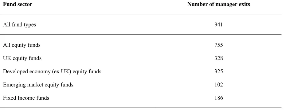
7 Table 1: Fund manager exits

This table contains a breakdown of the manager exits in our sample of funds over the period January 1997 to December 2011. These manager exits identified using predominantly Morningstar and Standard & Poor’s data, augmented by data from Citywire and Financial Express. These databases all cover UK mutual funds and provide information on fund management structures, investment objectives, fund benchmarks, fund managers’ characteristics and other fund characteristics.

Fund sector Number of manager exits

All fund types 941

All equity funds 755

UK equity funds 328

Developed economy (ex UK) equity funds 325 Emerging market equity funds 102 Fixed Income funds 186

The full sample includes both surviving and non-surviving funds and consists of 941fund manager

changes in total. 755 of the managers that leave their funds manage equity funds. Of this total 328

managed UK equity funds, 325 managed developed economy (ex UK) equity funds and 102

managed emerging market equity funds. Of the total 941 manager changes in our database 186

managed fixed income funds.

The price data for the funds and for their respective benchmarks was obtained from Morningstar

and covers the period from January 1994 (36 months prior to the first manager change in our

sample) to June 2014 (36 months after the last manager change in our sample). All of the funds in

which the change occurred were managed by a single manager, rather than by a team4_{. The}

Morningstar database identifies single manager and team managed funds. Our focus on single

manager managed funds should give a more precise idea of the impact of any manager change.

4 _{We excluded team managed funds as we would expect the effect of a change of the composition of a team to be less}

8 2.3 Normal and abnormal performance

The performance of the funds before and after the event date is measured using the

benchmark-adjusted model. We provide results for: all equity fund manager exits (Table 2); UK equity

managed fund manager exits (Table 3); developed economy (ex UK) fund manager changes (Table

4); emerging market equity fund manager changes (Table 5); and fixed income fund manager

changes (Table 6). For all manager exits and for each sample of these changes, we also

sub-divide the pre-exit performance of all funds and each sub-sample into either performance deciles or

into quintiles (depending upon the size of the sub-sample). By subdividing the data in this way we

hope to see whether the exit of, for example, a top performing manager had a different impact on

the subsequent performance of that fund compared with the exit of relatively poorly performing

manager from another fund.

The traditional event study methodology based on the market model requires that α’s and β’s are

estimated in a preliminary stage of the process. However, we concur with the views of Cremers et

al (2012), Argon and Ferson (2006) or Angelidis et al (2013), who all argue that it is more

informative and useful for investors and researchers if the performance of mutual fund managers is

measured against a passive benchmark which is closely aligned to a fund’s objectives and its risk

return parameters. A dedicated passive benchmark should provide a more accurate and more

appropriate estimate of a manager’s value-added skill. Given this, for our analysis we use the

benchmark-adjusted return model. This model can be thought of as a restricted market model

where α is equal to zero and where β is equal to one. We calculate benchmark-adjusted abnormal

returns as follows:

bt it

it R R

9 whereAR_itis the Abnormal Return of fund i in period t, R_itis the actual return of fund i in period t

and R_bt is the actual return of the benchmark for fund i in period t. We use the benchmark index

defined by the investment objectives of a fund to calculateR_bt. The information on fund

benchmarks is obtained from Morningstar, Citywire, S&P database or from fund fact sheets. t in

equation 1 represents event time, the manager exit occurs at t=0. In our analysis we define 36 to

t-1 (inclusive) as the pre-event window and t+t-1 to t+36 as the post event window.

We then use these ARs to eliminate any fund-specific bias by calculating Average Abnormal

Returns (AARs hereafter) for the whole sample and for any sub-sample of the funds, j:





 n

i it

jt AR

n AAR

1 1

(2)

where n is the number of funds for which the change of a fund manager has occurred. Additionally,

we also calculate Cumulative Average Abnormal Returns (CAARs) for various event windows of

size k, and for different groups of funds (j) as follows:





1

    



 _







k

t

jt

jt AR

CAAR (3)

We present the CAARs in graphical form.

2.4 Test statistics

Our tests focus on the average AARs produced by the funds over pre- and post-exit periods, where

10 quartiles, depending upon the size of the sample of funds5_{. The statistical significance of the}

various AARs that we calculate are based upon the test proposed in Brown and Warner (1985):

j j

σ

0 AAR

t  (4)

where AARj is the average AAR produced by the jth group of funds over either a pre-event

window from t-k to t-1, or the post event window from t+1 to t+k, where k is the event window; and

where _jis the standard deviation of the AARs produced by the same set of j funds estimated over

a comparable, pre-event period of k months:

1 )

( 2

1

 







 

k

AAR

AAR j

t

k t

jt

j



Equation (4) can tell us whether the average abnormal returns produced by a set of funds is

statistically different from zero or not, over any event window so that we can establish, for example,

whether funds that experience a fund manager exit then go on to produce significant, above

benchmark returns in subsequent periods.

We also employ another test which addresses a different, but related question. By comparing the

pre- and post-exit average AARs of any set of j funds we can establish whether manager exits

change the performance of the funds relative to their pre-exit performance. To do this we use the

standard t-test for the comparison of two means as follows:

5 _{In preliminary work we also calculated similar test statistics focussing on the CAARs of the funds, but the results were}

11





AAR AAR t -1 t to k t j, k t to 1 t j, -1 t to k t j, k t to 1 t j, / ) ( ) (        

 (6)

Effectively we subtract the average pre-event AARj, t1 to tk from the equivalent post event

k t to 1 t j,

AAR   sing the same event window k in both cases and then by calculating the variances of

these two sets of average returns we construct a t-test to establish whether the two means are

insignificantly different from one another. A positive and significant t-value indicates that average

returns were higher in the post-exit period than in the comparable pre-exit period.

2.5 Regression Analysis

It is well-documented in the literature that investing in small-capitalisation stocks (see for instance

Banz, 1981), value stocks (see Fama and French, 1992, among others) and winners (as in Jegadeesh

and Titman, 1993) earns higher risk-adjusted returns. It is possible then that a change in manager is

accompanied by a change in factor exposures. To add more insight into the factors that might be

playing a part in any change in performance following a manager exit we estimate a panel version

of Carhart’s (1997) four-factor model6 _{for all of the equity funds in our sample. In order to}

determine the impact of a manager change, we enhance the basic model with both intercept and

slope dummy variables, as shown in equation (7):

t i jt j D j jt j j D i i ft t

i R F F

R 4 _,

1 4 1 , ) (    





where R_i,tis the return on fund i in period t; t represents event time spanning 36 months before and

after the manager change, where the manager change occurs at t=0; R_ftis the risk free rate in period

t;



and in a panel setting represents the average sensitivity of the funds in the panel to the jth Carhart

6_{Hausman test is used to confirm the choice of a fixed compared with a random effects panel model. The chi-squared}

12 factor. The four factors are: the excess return on the market (R_m,t R_f,t), where Rm,tis the return

on a proxy for the market portfolio; Fama and French’s (1993) size (SMB) and style (HML) factors;

and Carhart’s (1997) momentum factor (MOM) factor. We then define a dummy variable, D,

which takes the value of 0 for the period t-36 to t=0 and the value of 1 for the period t=1 to t=36.

D i

 is a step dummy variable constructed as (_i D)and D j

 is an OLS coefficient on the

transformed factors, where the factors have been transformed as follows (DF_jt). The intercept

dummy D i

 provides a test for whether there is a significant improvement (or deterioration) in the

performance of funds following a manager change. The D j

 coefficients allow us to examine

whether a new manager changes a fund’s exposure to the market, size, value or momentum risk

factors. Since 427 out of 755 of the equity funds in our sample have an international focus (either

developed markets (ex UK) or emerging markets), we use global Fama-French-Carhart factors7 _in

the above model for these funds. For the 328 UK Equity Funds we apply Fama-French-Carhart UK

equivalent factors calculated by Gregory, Tharayan and Christides (2013)8_{. Since these factors are}

only relevant for equity funds only, we limit this regression analysis to the 755 equity funds in our

sample.

3. Results

We apply the methodology described in section 2 to the returns of funds that have experienced a

manager exit. Table 1 shows the decomposition of fund manager exits by both broad asset category

(equity and fixed income funds) and by equity fund sub-categories (UK equity, Global developed

equity (ex UK) and Emerging equity market funds).

7 _{Downloadable from http://mba.tuck.dartmouth.edu/pages/faculty/ken.french/data_library.html}

13 3.1 All equity fund manager exits

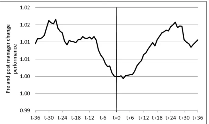
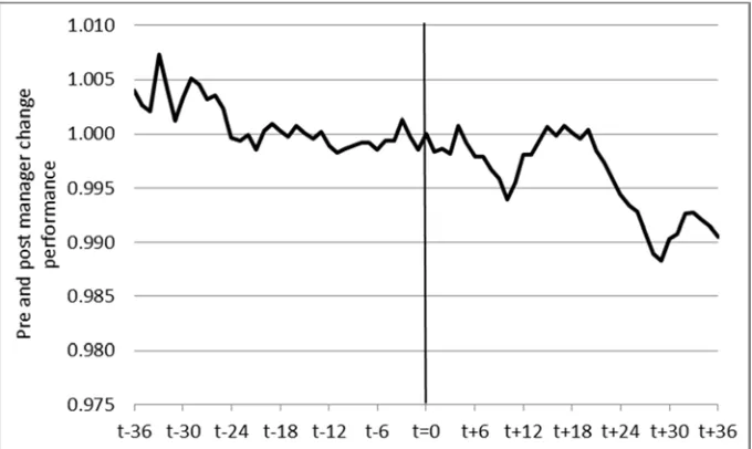
Figure 1 provides a simple, graphical summary of the cumulative 36 month, pre- and post-exit

performance of all equity funds that have suffered a manager exit over the sample period. The

graph is rebased to 1 at t=0; t-36 to t=0 shows the cumulative performance over this pre-manager

exit period, while t=0 to t+36 shows the cumulative performance after the manager change.

Figure 1: All equity funds

This figure shows the cummulative abnormal performance of all UK equity mutual funds that have experienced a manager exit over the period from January 1997 to December 2011. The horizontal axis represents event time; the manager exit occurs at t=0. The index of cumulative performance (vertical axis) is set equal to 1 at t=0.

The chart shows that the CAAR of this set of funds up to the manager exit was around -1.0%, which

means that on average this set of managers underperformed their benchmarks in the lead up to a

manager change. This is perhaps unsurprising and suggests that the predominant reason for a

manager exit is poor performance. However, perhaps surprisingly the chart also shows that, on

average, investors in these funds benefited from benchmark outperformance of up to 2.0% over the

24 months following the exit; but only around 1.0% after 36 months. These results are also

presented in Panel A of the first row of Table 2. In this row we present the AARs for all equity

mutual funds in our sample over six sample periods, three pre-exit and three post-exit. The

associated t-statistics test the hypothesis that the performance of these funds is significantly

14 sample periods is found to be insignificantly different from zero. For example, the average monthly

performance of the funds between t=1 and t=12 (inclusive) is 0.05%, but the associated t-statistic of

0.53, indicates that this is insignificantly different from zero.

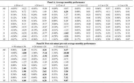
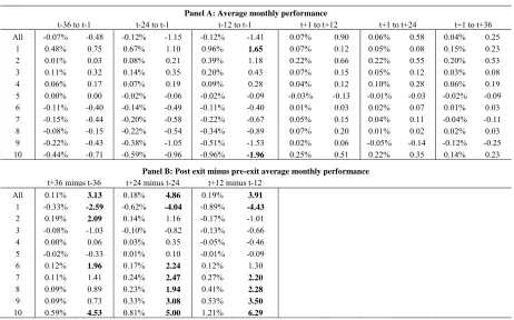
Table 2: All equity funds

This table presents the pre- and post-exit average monthly performance of all those equity mutual funds in the sample that experienced a manager exit between January 1997 and December 2011. The month of the manager exit is set to t=0. In Panel A the column headings refer to the event window used to calculate the average monthly returns and the associated statistic to establish whether the average is significantly different from zero (see equation 4). Those t-statistics that indicate significance at at least the 90% level of confidence are highlighted in bold for ease of reference. Each row in Panel A presents the results for all equity funds, and the results for the pre-exit performance deciles. These deciles were formed by calculating the pre-exit performance of each fund over the 12 months prior to the manager exit. The top ten per cent of funds comprise the decile 1, the next ten per cent decile 2, etc. The final three columns in the panel present the average returns of these same performance-ranked deciles of funds after the manager exit. Panel B in the Table presents the average monthly performance difference between all funds and the deciles, over three event windows. The associated t-statistics test for a significant difference between the post-exit and pre-exit average monthly performance (see equation 6).

Panel A: Average monthly performance

t-36 to t-1 t-24 to t-1 t-12 to t-1 t+1 to t+12 t+1 to t+24 t+1 to t+36 All -0.03% -0.22 -0.05% -0.50 -0.09% -0.97 0.05% 0.53 0.06% 0.57 0.03% 0.25

1 0.61% 0.72 1.01% 1.49 1.56% 4.29 0.00% 0.01 -0.07% -0.11 0.01% 0.01

2 0.14% 0.32 0.24% 0.49 0.53% 1.27 0.10% 0.23 0.01% 0.02 0.01% 0.02 3 0.12% 0.40 0.12% 0.42 0.25% 0.93 0.18% 0.66 0.10% 0.36 0.08% 0.26 4 0.13% 0.54 0.16% 0.59 0.08% 0.28 -0.06% -0.21 0.06% 0.22 0.05% 0.19 5 0.02% 0.13 -0.03% -0.17 -0.06% -0.34 -0.01% -0.05 0.03% 0.20 0.03% 0.14 6 -0.09% -0.35 -0.12% -0.47 -0.18% -0.77 0.03% 0.12 0.11% 0.43 0.05% 0.21 7 -0.10% -0.29 -0.19% -0.58 -0.31% -1.23 0.01% 0.05 0.05% 0.14 0.05% 0.14 8 -0.22% -0.59 -0.28% -0.77 -0.48% -2.03 0.08% 0.32 0.12% 0.33 0.12% 0.32 9 -0.24% -0.44 -0.51% -1.25 -0.78% -3.21 0.03% 0.11 -0.06% -0.16 -0.16% -0.30

10 -0.67% -0.76 -0.96% -1.11 -1.61% -3.22 0.17% 0.33 0.26% 0.30 0.06% 0.07

Panel B: Post exit minus pre-exit average monthly performance

t+36 minus t-36 t+24 minus t-24 t+12 minus t-12 All 0.06% 2.10 0.11% 4.34 0.15% 4.17

1 -0.60% -4.00 -1.08% -7.14 -1.56% -10.80

2 -0.13% -1.43 -0.24% -1.92 -0.44% -2.58

3 -0.04% -0.62 -0.02% -0.21 -0.07% -0.71 4 -0.09% -1.57 -0.10% -1.43 -0.14% -1.49 5 0.00% 0.04 0.06% 1.17 0.05% 0.69 6 0.14% 2.40 0.22% 3.44 0.21% 2.53

7 0.15% 1.98 0.23% 2.62 0.32% 3.20

8 0.34% 4.42 0.40% 4.34 0.55% 5.41

9 0.08% 0.68 0.44% 4.32 0.81% 7.32

10 0.73% 4.40 1.22% 6.28 1.77% 9.87

It is very possible of course that the performance of a fund after a manager has left will be heavily

influenced by the quality of the manager that left. It was not possible to discern the reason for a

manager exit from our databases mainly because fund management groups have a tendency to paint

any manager exit in as positive a light as possible! Most of the related press statements gave no

15 exit of a ‘good’ manager might have a different impact on the post-exit performance of a fund than

the exit of a ‘bad’ manager. To explore this possibility we split the sample of equity funds into

performance deciles. We created a top performing decile of funds that comprised the 10% of the

sample with the highest average pre-exit performance (from t-12 to t-1); the next decile comprised

the 10% of funds with the next best average performance over this period, etc. In Panel A of Table

2, we have presented the pre and post exit performance of each of these deciles. By construction

the table shows that decile 1 outperformed their benchmarks before the exit and that this

outperformance gradually declines as we move from decile 1 to 10. For example, we find that the

average monthly return of deciles 1 and ten over the 36 months prior to the exit event, is 0.61% and

-0.67% respectively. For both the 36 month and 24 month pre-exit periods, the t-statistics lead us to

conclude that this average, pre-exit benchmark-adjusted performance is nearly always

indistinguishable from zero. However, this is not the case when we consider the 12 month period

before the exit. First the average outperformance of those managers that comprise decile 1 is found

to be highly statistically significant. Second, the average underperformance of managers that

comprise deciles, 8, 9 and 10 is found to be statistically significant.

Of more interest, however, is the post-exit performance of these funds. The columns in Panel A of

Table 2 headed t+12, t+24 and t+36 present the post-exit, average performance of the deciles

respectively, along with the statistical significance of this performance in the respective, adjacent

columns. Over the first 12 months decile 1, produces an average underperformance of 0.00%.

Indeed most of the other deciles either produce an economically small outperformance over this

period, or underperform. But overall, the average outperformance for all equities is 0.05% over

this period. It is clear where this comes from when we focus on decile 10. The average

benchmark-adjusted performance of decile ten is estimated to be 0.17% over the first twelve

months; however, the associated t-statistic of 0.33 indicates that this result is not statistically

16 also not found to be statistically significant. These results suggest that over the first 12 months

following a manager exit, fund performance tends to deteriorate for most funds, but tends to

improve in those instances where the manager was a bottom decile performer prior to the exit.

Panel B of Table 2 presents answers to a different question. Using equation 6 we test for a

significant change in the pre- and post-exit performance of all funds and each decile of funds. The

column headed “t+36–t-36”, compares 36 month post-exit performance with 36 month pre-exit

performance. The columns headed “t+24–t-24” and “t+12–t-12” compare performance over

equivalent 24 and 12 month periods. The associated t-statistics are based on equation 6, and

essentially test whether the average pre- and post-exit performances are significantly different from

one another. Essentially we are asking whether there has been a change in the benchmark-adjusted

performance of the funds following a manager exit. The t-statistics in the first row of Panel B

shows that there is indeed a positive structural change in the benchmark-adjusted performance of

UK mutual funds following a manager exit over all three event sample periods. For example over

the 12 months following a manager exit, on average, investors are 0.15% per month than they were

over the 12 months prior to the exit. However, when we consider the performance deciles we find

that those investors in deciles 1 to 4 experience a decline in performance over all three sample

periods. When comparing the 12 months before and after the manager exit, those investors in decile

1 experience an average deterioration of 1.56% per month over the 12 post-exit months; a result that

is found to be highly statistically significant. At the other end of the scale investors in decile 6 to 10

all experience a statistically significant improvement in monthly performance over the 12 post exit

months, ranging from 0.21% per month to 1.77% per month for decile 10. The positive relative

improvement in all funds shown in the first row of Panel B of Table 2, indicates that on average the

post-exit deterioration in performance of funds that were performing well before the manager exit is

more than offset by the post-exit improvement in the performance of managers that were

17 The results in this section apply to all of the equity funds in our sample, but it is possible that the

results presented here were influenced by the equity sectors in which the managers operated. In

sections 3.2 to 3.4, we apply the same manager exit analysis to UK equity, Developed Economy

equity (ex UK) and emerging market funds.

3.2 UK equity fund manager exits

In Figure 2 we present the post exit performance of all 328 UK equity funds, the performance and

statistics of this set of funds is presented in Table 3.

Figure 2: UK equity funds

This figure shows the cummulative abnormal performance of all those UK mutual funds comprising UK equities that have experienced a manager exit over the period from January 1997 to December 2011. The horizontal axis represents event time; the manager exit occurs at t=0. The index of cumulative performance (vertical axis) is set equal to 1 at t=0.

The figure shows that over the 36 months prior to the manager exit the average,

benchmark-adjusted cumulative performance was -2.80% so, on average these managers were underperforming

their benchmarks before they left their funds. The average post-exit performance is very similar to

that for all equity funds shown in Figure 1. Over the 36 post-exit months the average,

benchmark-adjusted performance is just over 1.5%. This result suggests that on average, investors in UK

18 Table 3 indicates that both the pre- and post-exit performance over all three event windows, is never

significantly different from zero at conventional confidence levels.

Table 3: UK equity funds

This table presents the pre- and post-exit average monthly performance of all those equity mutual funds in the sample that experienced a manager exit between January 1997 and December 2011. The month of the manager exit is set to t=0. In Panel A the column headings refer to the event window used to calculate the average monthly returns and the associated statistic to establish whether the average is significantly different from zero (see equation 4). Those t-statistics that indicate significance at at least the 90% level of confidence are highlighted in bold for ease of reference. Each row in Panel A presents the results for all UK equity funds, and the results for the pre-exit performance deciles. These deciles were formed by calculating the pre-exit performance of each fund over the 12 months prior to the manager exit. The top ten per cent of funds comprise the decile 1, the next ten per cent decile 2, etc. The final three columns in the panel present the average returns of these same performance-ranked deciles of funds after the manager exit. Panel B in the Table presents the average monthly performance difference between all funds and the deciles, over three event windows. The associated t-statistics test for a significant difference between the post-exit and pre-exit average monthly performance (see equation 6).

Panel A: Average monthly performance

t-36 to t-1 t-24 to t-1 t-12 to t-1 t+1 to t+12 t+1 to t+24 t+1 to t+36 All -0.07% -0.48 -0.12% -1.15 -0.12% -1.41 0.07% 0.90 0.06% 0.58 0.04% 0.25

1 0.48% 0.75 0.67% 1.10 0.96% 1.65 0.07% 0.12 0.05% 0.08 0.15% 0.23

2 0.01% 0.03 0.08% 0.21 0.39% 1.18 0.22% 0.66 0.22% 0.55 0.20% 0.53 3 0.11% 0.32 0.14% 0.35 0.20% 0.43 0.07% 0.15 0.05% 0.12 0.03% 0.08 4 0.06% 0.17 0.07% 0.19 0.09% 0.28 0.04% 0.12 0.10% 0.28 0.06% 0.19 5 0.00% 0.00 -0.02% -0.06 -0.02% -0.09 -0.03% -0.13 -0.01% -0.03 -0.02% -0.09 6 -0.11% -0.40 -0.14% -0.49 -0.11% -0.40 0.01% 0.03 0.02% 0.07 0.01% 0.03 7 -0.15% -0.44 -0.20% -0.58 -0.22% -0.67 0.05% 0.15 0.04% 0.11 -0.04% -0.11 8 -0.08% -0.15 -0.22% -0.54 -0.34% -0.89 0.07% 0.20 0.01% 0.02 0.02% 0.03 9 -0.22% -0.43 -0.38% -1.05 -0.51% -1.53 0.02% 0.06 -0.05% -0.14 -0.12% -0.25 10 -0.44% -0.71 -0.59% -0.96 -0.96% -1.96 0.25% 0.51 0.22% 0.35 0.14% 0.23

Panel B: Post exit minus pre-exit average monthly performance

t+36 minus t-36 t+24 minus t-24 t+12 minus t-12 All 0.11% 3.13 0.18% 4.86 0.19% 3.91

1 -0.33% -2.59 -0.62% -4.04 -0.89% -4.43

2 0.19% 2.09 0.14% 1.16 -0.17% -1.01

3 -0.08% -1.03 -0.10% -0.82 -0.13% -0.66 4 0.00% 0.06 0.03% 0.35 -0.05% -0.46

5 -0.02% -0.33 0.01% 0.10 -0.01% -0.09

6 0.12% 1.96 0.17% 2.24 0.12% 1.30

7 0.11% 1.41 0.24% 2.47 0.27% 2.20

8 0.09% 0.89 0.23% 1.94 0.41% 2.28

9 0.09% 0.73 0.33% 3.08 0.53% 3.50

10 0.59% 4.53 0.81% 5.00 1.21% 6.29

However, once again the first row of Panel B in Table 3 shows that there was a highly statistically

significant positive improvement in 12, 24 and 36 month post exit performance. For example, the

average performance of the UK equity funds over the 12 months following the manager exit was

0.19% per month higher than the average over the 12 months prior to the exits; the t-test of 3.91,

19 Panels A and B of Table 3 also present the performance statistics for the UK equity fund pre- and

post-exit performance deciles. The positive performance for all funds from t+1 to t+12 is again

heavily dominated by decile 10’s performance. The average benchmark outperformance of the

worst pre-exit performers between t+1 and t+12 is 0.25%. However, the performances pre- and

post-exit, over all event periods, are rarely found to be statistically different from zero. However,

Panel B of the table indicates again that post-exit performance is significantly different from the

pre-exit performance for all funds, over all three event window comparisons. The results for decile

1 indicate a significant deterioration in the performance of the funds that were top performers

before the manager exit of -0.89% per month, while at the other extreme we find that deciles 7 to 10

(particular for the 12 month comparator) produce improved performance which is statistically

significant following the manager exits over all three monitoring periods. The results for the mutual

funds consisting of UK equities are therefore qualitatively similar to those results presented for all

equity funds in Table 2.

3.3 Developed economy equity fund manager exits (ex UK)

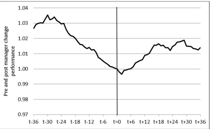
In Figure 3 we present the average pre- and post-exit performance for the subset of funds comprised

of developed economy equities (ex UK). Over the 36 month period prior to the manager exits the

funds produce an average, cumulative benchmark-adjusted performance of around -1.0%. The

pre-exit performance is also less stable, perhaps reflecting the mix of equity funds represented in the

sample. The figure also shows that the average post-exit performance is again positive; after 20

20 Figure 3: Global developed equity funds (ex UK)

This figure shows the cummulative abnormal performance of all those UK mutual funds comprising developed economy equities (ex UK) that have experienced a manager exit over the period from January 1997 to December 2011. The horizontal axis represents event time; the manager exit occurs at t=0. The index of cumulative performance (vertical axis) is set equal to 1 at t=0.

The first row in Panel A of the Table 4 shows that the post-exit performance is not statistically

significantly different from the performance of the benchmarks. However, row 1 of Panel B in the

Table 4 indicates that the post-exit performance is an improvement on the equivalent pre-exit

performance though only significantly so for the 24 and 12 month comparators. For example, the

average 12 month outperformance of the funds after the exits compared with before the exits is

0.16%, where the associated t-ratio for the test of the difference in the two means is 2.53.

Table 4 also contains the performance of the fund deciles. The post-exit performance of decile 10 is

the largest contributor to the positive average presented in row 1 of Panel A. Panel B shows that

there is a significant post-exit improvement in the performance of managers that managed funds in

the bottom two pre-exit performance deciles. This improvement is also evident for the funds that

comprise deciles 6 to 8 too, over 12 and 24 months after the manager exit. These results again

indicate that the manager exit is a significant event for a mutual fund, with top performing funds 0.99

1.00 1.00 1.01 1.01 1.02 1.02

t‐36 t‐30 t‐24 t‐18 t‐12 t‐6 t=0 t+6 t+12 t+18 t+24 t+30 t+36

Pr

e

and

Pos

t

ma

n

ager

ch

an

ge

pe

rf

or

m

an

21 suffering from poorer performance after the manager leaves and the bottom performers enjoying an

improvement in performance.

Table 4: Developed economy equity funds (ex UK)

This table presents the pre- and post-exit average monthly performance of all those developed economy equity mutual funds (ex UK) in the sample that experienced a manager exit between January 1997 and December 2011. The month of the manager exit is set to t=0. In Panel A the column headings refer to the event window used to calculate the average monthly returns and the associated t-statistic to establish whether the average is significantly different from zero (see equation 4). Those t-statistics that indicate significance at at least the 90% level of confidence are highlighted in bold for ease of reference. Each row in Panel A presents the results for all developed economy equity funds (ex UK), and the results for the pre-exit performance deciles. These deciles were formed by calculating the pre-exit performance of each fund over the 12 months prior to the manager exit. The top ten per cent of funds comprise the decile 1, the next ten per cent decile 2, etc. The final three columns in the panel present the average returns of these same performance-ranked deciles of funds after the manager exit. Panel B in the Table presents the average monthly performance difference between all funds and the deciles, over three event windows. The associated t-statistics test for a significant difference between the post-exit and pre-exit average monthly performance (see equation 6).

Panel A: Average monthly performance

t-36 to t-1 t-24 to t-1 t-12 to t-1 t+1 to t+12 t+1 to t+24 t+1 to t+36 All -0.03% -0.14 -0.04% -0.22 -0.10% -0.67 0.05% 0.36 0.05% 0.25 0.02% 0.09

1 0.72% 0.62 1.23% 1.32 1.96% 3.35 0.01% 0.01 -0.16% -0.17 -0.14% -0.12

2 0.26% 0.51 0.40% 0.78 0.71% 1.92 0.20% 0.54 0.03% 0.05 0.05% 0.10

3 0.04% 0.07 0.11% 0.19 0.30% 0.65 0.11% 0.23 0.01% 0.01 0.02% 0.03 4 0.19% 0.32 0.21% 0.33 0.06% 0.12 -0.09% -0.18 -0.02% -0.03 0.04% 0.06 5 0.09% 0.20 -0.07% -0.16 -0.09% -0.20 0.12% 0.26 0.08% 0.17 0.10% 0.22 6 -0.17% -0.39 -0.15% -0.39 -0.21% -0.47 0.02% 0.04 0.12% 0.32 0.07% 0.15 7 -0.19% -0.33 -0.22% -0.35 -0.36% -0.92 0.03% 0.07 0.15% 0.23 0.09% 0.15 8 -0.35% -0.68 -0.40% -0.75 -0.53% -1.89 0.06% 0.21 0.14% 0.26 0.12% 0.23 9 -0.29% -0.42 -0.54% -0.80 -0.87% -1.49 0.04% 0.07 -0.18% -0.27 -0.27% -0.38 10 -0.39% -0.36 -0.62% -0.52 -1.50% -1.79 -0.09% -0.11 0.31% 0.26 0.11% 0.10

Panel B: Post exit minus pre-exit average monthly performance

t+36 minus t-36 t+24 minus t-24 t+12 minus t-12 All 0.04% 1.08 0.09% 1.89 0.16% 2.53

1 -0.86% -3.98 -1.39% -6.18 -1.95% -8.30

2 -0.21% -1.54 -0.37% -2.06 -0.51% -1.90

3 -0.02% -0.17 -0.10% -0.70 -0.20% -1.05 4 -0.16% -1.35 -0.23% -1.59 -0.15% -0.93 5 0.01% 0.10 0.15% 1.26 0.21% 1.21

6 0.24% 2.22 0.27% 2.22 0.23% 1.46

7 0.28% 2.22 0.37% 2.30 0.39% 2.41

8 0.47% 3.89 0.54% 3.85 0.59% 3.96

9 0.02% 0.16 0.36% 2.00 0.91% 4.09

10 0.50% 2.21 0.93% 3.10 1.40% 4.75

3.4 Emerging market equity fund manager exits

Figure 4 and Table 5 presents the results for the emerging market funds in our data set. Figure 4

appears to be quite different from figures 1, 2 and 3. As Figure 4 shows, the average pre-exit

performance is positive over the 36, 24 and 12 month periods leading up to a manager exit. In other

words the average manager of emerging market equities was ahead of benchmark before their exit.

This result possibly explains why the average post-exit performance is approximately 0.00% over

22 or post-exit managers do not produce a benchmark-adjusted performance that is significantly

different from zero over any timeframe. However, in contrast to the results in tables 2, 3 and 4, the

first row of panel B in the table indicate that on average, there is no significant structural break that

occurs following an emerging equity manager exit.

Figure 4: Emerging market equity funds

This figure shows the cummulative abnormal performance of all those UK mutual funds comprising emerging market equities that have experienced a manager exit over the period from January 1997 to December 2011. The horizontal axis represents event time; the manager exit occurs at t=0. The index of cumulative performance (vertical axis) is set equal to 1 at t=0.

Because the sample of funds is relatively small, rather than splitting their pre- and post-exit

performance into pre-exit performance deciles, instead we split the performance into pre-exit

performance quintiles. Although Panel A of Table 5 shows that generally the performance of

outperforming funds prior to a manager exit deteriorates after the exit and that the converse is true

for underperforming funds, the results in this Panel show that these average performance statistics

are never statistically significant from zero over any performance sample.

The t-statistics in Panel B of the table indicate that there is a significant structural break in the

performance of quintile 1 over all three periods analysed. For example, on average investors in

quintile 1 suffer a deterioration in performance of -0.54% per month over the 36 post-manager exit

months, compared to the 36 months prior to the exit. At the other end of the scale we find that 0.92

0.94 0.96 0.98 1.00 1.02 1.04

t‐36 t‐30 t‐24 t‐18 t‐12 t‐6 t=0 t+6 t+12 t+18 t+24 t+30 t+36

Pr

e

and

pos

t

ma

na

ge

r

ch

ange

pe

rf

o

rm

an

23 investors in quintile 1 would have experienced an average improvement in performance of 1.05%,

0.76% and 0.31% over the 12, 24 and 36 month post exit months compared to the equivalent

pre-exit months; although we only find these averages to be statistically different from one another over

the 12 and 24 month periods.

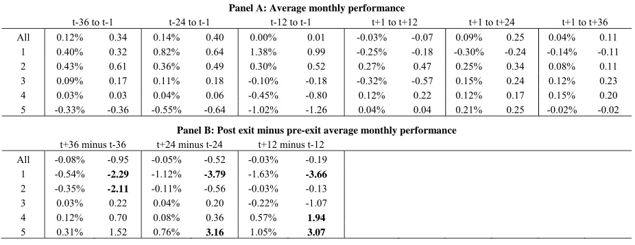
Table 5: Emerging market equity funds

This table presents the pre- and post-exit average monthly performance of all those emerging market equity mutual funds in the sample that experienced a manager exit between January 1997 and December 2011. The month of the manager exit is set to t=0. In Panel A the column headings refer to the event window used to calculate the average monthly returns and the associated t-statistic to establish whether the average is significantly different from zero (see equation 4). Those t-statistics that indicate significance at at least the 90% level of confidence are highlighted in bold for ease of reference. Each row in Panel A presents the results for all emerging market equity funds, and the results for the pre-exit performance quintiles. These quintiles were formed by calculating the pre-exit performance of each fund over the 12 months prior to the manager exit. The twenty per cent of funds comprise quintile 1, the next twenty per cent quintile 2, etc. The final three columns in the panel present the average returns of these same performance-ranked quintiles of funds after the manager exit. Panel B in the Table presents the average monthly performance difference between all funds and the quintiles, over three event windows. The associated t-statistics test for a significant difference between the post-exit and pre-exit average monthly performance (see equation 6).

Panel A: Average monthly performance

t-36 to t-1 t-24 to t-1 t-12 to t-1 t+1 to t+12 t+1 to t+24 t+1 to t+36 All 0.12% 0.34 0.14% 0.40 0.00% 0.01 -0.03% -0.07 0.09% 0.25 0.04% 0.11

1 0.40% 0.32 0.82% 0.64 1.38% 0.99 -0.25% -0.18 -0.30% -0.24 -0.14% -0.11 2 0.43% 0.61 0.36% 0.49 0.30% 0.52 0.27% 0.47 0.25% 0.34 0.08% 0.11 3 0.09% 0.17 0.11% 0.18 -0.10% -0.18 -0.32% -0.57 0.15% 0.24 0.12% 0.23 4 0.03% 0.03 0.04% 0.06 -0.45% -0.80 0.12% 0.22 0.12% 0.17 0.15% 0.20 5 -0.33% -0.36 -0.55% -0.64 -1.02% -1.26 0.04% 0.04 0.21% 0.25 -0.02% -0.02

Panel B: Post exit minus pre-exit average monthly performance

t+36 minus t-36 t+24 minus t-24 t+12 minus t-12 All -0.08% -0.95 -0.05% -0.52 -0.03% -0.19

1 -0.54% -2.29 -1.12% -3.79 -1.63% -3.66

2 -0.35% -2.11 -0.11% -0.56 -0.03% -0.13

3 0.03% 0.22 0.04% 0.20 -0.22% -1.07

4 0.12% 0.70 0.08% 0.36 0.57% 1.94

5 0.31% 1.52 0.76% 3.16 1.05% 3.07

3.5 Fixed income fund manager exits

The performance of fixed income mutual funds is much neglected in the academic literature,

although there are some notable exceptions. Given that one would expect the performance of fixed

income and equity funds to be of a different scale we have separated the 186 fixed income funds

that experienced a manager exit over the sample period from the equity funds. Figure 5 shows the

average pre- and post-exit performance of the fixed income funds in our sample. The profile and

scale is very different from the one identified for developed economy equities. On average the

24 post-exit assessment period the abnormal performance was very flat; after 36 post-event months the

average cumulative underperformance is -0.10%.

Figure 5: Fixed income funds

This figure shows the cummulative abnormal performance of all those UK mutual funds comprising fixed income securities (bonds) that have experienced a manager exit over the period from January 1997 to December 2011. The horizontal axis represents event time; the manager exit occurs at t=0. The index of cumulative performance (vertical axis) is set equal to 1 at t=0.

Row 1 in Panel A of Table 6 shows that the average pre and post-exit performance is both

economically small and is insignificant different from zero. The first row of Panel B in Table 6 also

suggests that on average there is no significant change in pre- and post-exit performance; a result

that is in contrast to the results for the equity funds in our sample.

Panel A shows that the average returns of the deciles across all of the event window periods are

almost never significantly different from zero (the one exception being the 12 month pre-manager

exit average for decile 10). However, when we consider the post-exit performance with the pre-exit

performance we again find that the manager exit has had a significant impact on the performance

extremes. However, Panel B shows that there is a significant deterioration in the performance of

decile 1 over all three sample periods. For example, the average return for this decile of funds is

0.46% lower in the 36 months after the manager exits than it was in the 36 months before the exits.

25 other end of the scale, over all three sample periods, we find that there is an average improvement

in performance after the manager exit for deciles 8 to 10. For example, for decile 10 the average

performance improvement during the first 12 months following the manager exit compared to the

12 months prior to the exit is 1.04% per month, a result that has an associated t-value of 3.70.

Table 6: Fixed income funds

This table presents the pre- and post-exit average monthly performance of all those fixed income mutual funds in the sample that experienced a manager exit between January 1997 and December 2011. The month of the manager exit is set to t=0. In Panel A the column headings refer to the event window used to calculate the average monthly returns and the associated statistic to establish whether the average is significantly different from zero (see equation 4). Those t-statistics that indicate significance at at least the 90% level of confidence are highlighted in bold for ease of reference. Each row in Panel A presents the results for all fixed income funds, and the results for the pre-exit performance quintiles. These quintiles were formed by calculating the pre-exit performance of each fund over the 12 months prior to the manager exit. The twenty per cent of funds comprise quintile 1, the next twenty per cent quintile 2, etc. The final three columns in the panel present the average returns of these same performance-ranked quintiles of funds after the manager exit. Panel B in the Table presents the average monthly performance difference between all funds and the quintiles, over three event windows. The associated t-statistics test for a significant difference between the post-exit and pre-exit average monthly performance (see equation 6).

Panel A: Average monthly performance

t-36 to t-1 t-24 to t-1 t-12 to t-1 t+1 to t+12 t+1 to t+24 t+1 to t+36 All -0.01% -0.07 0.00% 0.01 0.01% 0.08 -0.02% -0.15 -0.02% -0.24 -0.03% -0.17

1 0.44% 0.47 0.79% 0.90 1.14% 1.58 -0.30% -0.41 -0.22% -0.26 -0.02% -0.02 2 0.26% 0.38 0.32% 0.48 0.40% 0.65 0.24% 0.38 0.08% 0.11 0.09% 0.13 3 0.04% 0.09 0.13% 0.31 0.14% 0.29 0.13% 0.27 0.11% 0.28 0.04% 0.10 4 -0.07% -0.23 -0.06% -0.16 0.00% 0.01 0.03% 0.07 0.00% 0.00 0.01% 0.03 5 0.01% 0.02 -0.03% -0.05 -0.06% -0.21 0.05% 0.17 0.01% 0.01 0.00% 0.01 6 -0.11% -0.40 -0.03% -0.15 -0.11% -0.53 -0.23% -1.10 -0.12% -0.62 -0.12% -0.44 7 0.02% 0.01 -0.29% -0.37 -0.17% -0.31 -0.10% -0.17 -0.14% -0.18 -0.12% -0.11 8 -0.35% -0.68 -0.26% -1.05 -0.33% -1.38 -0.12% -0.49 -0.10% -0.41 -0.06% -0.12 9 -0.28% -0.53 -0.42% -0.85 -0.60% -1.31 0.01% 0.03 0.03% 0.05 -0.07% -0.13 10 -0.17% -0.22 -0.43% -0.61 -0.92% -2.06 0.11% 0.26 0.23% 0.32 0.08% 0.10

Panel B: Post exit minus pre-exit average monthly performance

t+36 minus t-36 t+24 minus t-24 t+12 minus t-12 All -0.02% -0.45 -0.02% -0.72 -0.02% -0.44

1 -0.46% -2.35 -1.01% -4.42 -1.44% -4.93

2 -0.17% -1.04 -0.25% -1.20 -0.16% -0.50

3 0.00% 0.04 -0.01% -0.11 -0.01% -0.06

4 0.08% 1.19 0.06% 0.59 0.03% 0.18

5 -0.01% -0.06 0.03% 0.22 0.11% 0.85

6 -0.01% -0.14 -0.09% -1.27 -0.12% -1.07

7 -0.14% -0.65 0.14% 0.70 0.08% 0.32

8 0.29% 2.97 0.16% 2.50 0.21% 2.26

9 0.21% 1.90 0.45% 3.78 0.61% 3.79

10 0.25% 1.43 0.66% 3.19 1.04% 3.70

4. Changing factor exposures

The results from our event study presented in section 3 of this paper show that a manager change,

26 regressions based on equation (7) for each set of equity funds in our sample: All equity funds, UK

equities, Global Developed (ex UK) and Emerging Markets. The second column in Table 7

presents the regression results for all of the equity funds in our sample. The positive and highly

statically significant value estimated for the coefficient on _D _{indicates that even in the presence of}

the four risk factors that there is an average improvement in post manager exit alpha of 0.15% per

month over the three years following an exit. The coefficients on the transformed risk factors

(superscript D) indicate a significant decline in exposure to the market and a significant increase

exposure to the value (HML) and momentum (MOM) factors. The negative value for the

coefficient on SMBD _{indicates a reduction in exposure to small stocks, but the coefficient is found}

to be both economically small (-0.02) and insignificantly different from zero. The changes in the

exposures to alpha and the risk factors for UK equities shown in column 3 are almost identical to

those found for all equity funds. However, the coefficients on the transformed variables are

smaller. For example, we find a significant improvement in post manager exit alpha of 0.10% per

month as opposed to the 0.15% per month for all equity funds. Furthermore, although the

coefficient on SMBD _{is still economically small (-0.03) it is now statistically significant. In column}

4 in the Table we present the results for the Global Developed (ex UK) equity funds. The results

for these funds are broadly consistent with those of the UK equities fund sample, but we find a

more economically significant shift to the value and Momentum factors. This is most notable in the

former where the coefficient on HMLD _{is found to be 0.24%. The results for the Emerging market}

equities funds are different from the results for the other funds. First we estimate that the change in

manager had, on average, a negative impact on subsequent fund alpha, although this result is not

significant at conventional confidence levels. Second, there is a slight, but again insignificant,

increase in exposure to the market factor. Finally, there is an increase in exposure to the small stock

27 Table 7: Impact of manager change on fund risk factors

This table reports the results of the estimation of equation (7) in the text:

t i jt j j jt j j i i ft t

i R F F

R 4 _,

1 * 4 1 * , ) (    





For an explanation of the equation please see the related text in section 2.5. The first column in the table presents the variables in equation (7). The rows in the table Market, SMB, HML and MOM refer to the Carhart factors; the superscript D refers to the transformed version of the variable, where the transformation is achieved by multiplying the variable by a dummy variable D, which takes the value of 0 between t=-36 to t=0 and 1 from t=1 to t=36. Columns 2 to 5 present the coefficient values on the variables listed in column 1 for: All equity funds; UK equity funds; Global Developed (ex UK) funds; and Emerging Market funds respectively. We used global FF-Carhart risk factors for all samples (see footnote 7 in the text), except for the UK equities fund sample where we used UK equivalents (see footnote 8 in the text). The superscripts *, ** and *** denote the statistical significance of each coefficient at the 1%, 5% and 10% level respectively. The number of funds that made up the regression in each case is shown in the penultimate row of the table, while the R2 _{of each regression is presented in the last row of the table.}

Variable All funds UK

Global Developed (ex UK)

Emerging Markets

)

(



(

_

0.15* 0.10* 0.10*** -0.08

Market 0.87* 0.98* 0.85* 0.81* MarketD _{-0.06* -0.02* -0.07* 0.03}

SMB 0.24* 0.30* 0.18* 0.24* SMBD _{-0.02 -0.03* -0.02 0.14**}

HML -0.11* -0.06* -0.16* -0.40* HMLD _{0.10* 0.09* 0.24* 0.13**}

MOM -0.03* 0.04* -0.03* 0.02

MOMD _{0.06* 0.03* 0.08* 0.02}

Number of funds 755 328 325 102 R-squared 0.58 0.78 0.52 0.43

5. Summary and conclusions

This paper examines how the performance of UK mutual funds is affected when the incumbent fund

manager leaves the fund. When we focus on all equity mutual fund manager exits in the UK, we

find a significant impact on the post-exit performance of funds. Over the first 12 months following

an exit the average fund outperforms its benchmark. These results therefore suggest that a manager

exit is good for a fund’s performance on average. However, closer inspection of the funds by

pre-manager exit performance decile/quintile reveals that a fund that is a top performer prior to an exit

tends to suffer significant performance deterioration as a result of the exit, while the performance of

28 performance of the pre-exit poor performers that drives the average result. Our disaggregated

results indicate that a manager exit tends to have a negative impact on funds that were performing

well before the exit, but a positive effect on those that were previously underperforming.

When we separated the funds by sector we found that the results for those funds comprising UK

equities and, separately, those funds containing developed economy equities (ex UK) were

qualitatively similar to the aggregated results. However, the results for the emerging market equity

funds are different from those of the developed equity equivalents. Monthly abnormal performance

was generally positive before the manager exits and, on average, was virtually zero over the 36

post-event months. In addition, the top performing quintile produces a significant negative

performance over the post event months, in contrast to the positive post-exit performance of the top

deciles of developed economy equity funds. Although the quintile results are based on a relatively

small sample, the results for all emerging equity funds are still produced by a large enough sample

(63) to draw meaningful conclusions. It is possible that the emerging market and developed

economy equity market exits had, on average, different roots. Developed economy managers

generally underperformed before an exit, emerging market managers generally outperformed. It is

possible that over the period studied here, when more and more investors were becoming interested

in investing in emerging markets, that there was a bidding war between fund management firms for

the best emerging market managers, while developed economy manager exits were largely driven

by underperformance.

We also examined the impact of a manager exit on the performance of UK mutual funds comprising

fixed income securities. The overall results for the bond funds are similar to those for the emerging

equity market funds: average pre-exit performance is positive (more so for the fixed income funds

than for the emerging equity market funds) and the post exit performance is flat, although this

29 a significant impact on the performance of funds that were performing well and those that were

performing relatively badly; the formers’ performance deteriorates while the latters’ improves

significantly.

Finally, our regression analysis supports and reinforces the event study analysis in this paper,

showing that on average the fund manager replacements in our sample benefited investors. Our

regression results show that the improvement in performance is accompanied by a reduction in

market risk, a slight reduction in exposure to small cap risk, and an increase in exposure to value

stocks (via the HML risk factor) and momentum stocks (via the MOM risk factor). These results

are consistent with those of other researchers, such as Asness, Moskowitz and Pedersen (2013),

who find that combining value and momentum strategies leads to higher risk-adjusted returns. The

main exception to these findings is the decline in manager alpha documented for emerging market

equity funds.

Overall, our results suggest that UK fund management companies have been relatively successful in

replacing bad managers with better managers, but relatively unsuccessful at finding equivalent

replacements for their top performing managers. As such, we believe that regulators should ensure

that all efforts are made by fund management companies to inform all of their investors about a

30

References

Angelidis, T., Giamouridis, D., Tessaromatis, N., (2013), Revisiting mutual fund performance evaluation. Journal of Banking and Finance, 37(5), 1759–1776.

Asness, C.J., Moskowitz T.J and L.H Pedersen, (2013), Value and Momentum Everywhere, Journal of Finance, 68, 929-985.

Banz, R.W., (1981), The Relationship between Return and Market Value of Common Stocks, Journal of Financial Economics, 9, 3-18.

Blake, C.R. and Morey M.R., (2000), Morningstar ratings and mutual fund performance, Journal of Quantitative and Financial Analysis, 35(03), 451-483.

Bessler, W., Blake, D., Lückoff, P. and Tonks, I., (2010). Why does mutual fund performance not persist? The Impact and Interaction of Fund Flows and Manager Changes, Pensions Institute discussion paper, PI-1009

Brown, S.J. and Goetzmann, W.N., (1995), Performance Persistence, Journal of Finance, 2, 679-699.

Brown, S.J., and Warner, J., (1985), Using daily stock returns: The case of event studies, Journal of Financial Economics,14, 3-31.

Carhart, M.M., (1997), On Persistence in Mutual Fund Performance, Journal of Finance, 1, 57-83.

Chevalier, J. and Ellison, G., (1999), Are Some Mutual Fund Managers Better Than Others? Cross-Sectional Patterns in Behavior and Performance, Journal of Finance, 3, 875-899.

Cremers, M., Petajisto, A., Zitzewtz, E., (2012). Should benchmark indices have alpha? Revisiting performance evaluation. Critical Finance Review, 2, 1-48.