City, University of London Institutional Repository
Citation
:
Boscolo, M. and Banerjee, J. R. (2014). Layer-wise dynamic stiffness solution for free vibration analysis of laminated composite plates. Journal of Sound and Vibration, 333(1), pp. 200-227. doi: 10.1016/j.jsv.2013.08.031This is the accepted version of the paper.
This version of the publication may differ from the final published
version.
Permanent repository link: http://openaccess.city.ac.uk/14356/
Link to published version
:
http://dx.doi.org/10.1016/j.jsv.2013.08.031Copyright and reuse:
City Research Online aims to make research
outputs of City, University of London available to a wider audience.
Copyright and Moral Rights remain with the author(s) and/or copyright
holders. URLs from City Research Online may be freely distributed and
linked to.
Layer wise dynamic stiffness solution for free vibration
analysis of laminated composite plates
M. Boscolo∗
, J. R. Banerjee
School of Engineering and Mathematical Sciences, City University London, Northampton Square, London, EC1V 0HB
Abstract
The dynamic stiffness method has been developed by using a sophisticated layer wise theory which complies with theC0
z requirements and delivers high accuracy for the analysis of laminated composite plates. The method is ver-satile as it derives the dynamic stiffness matrix for plates with any number of layers in a novel way without the need to re-derive and re-solve the equations of motion when the number of layers has changed. This novel procedure to manipulate and solve the equations of motion has been referred to as the L-matrix method in this paper. The Carrera unified formulation (CUF) is employed to derive the equations of motion of a plate through the use of a first order layer wise assumption for a plate with a single layer first. The method is then generalised and extended to multiple layers. Essentially by writing the equations of motion of one single layer in the L-matrix form, the system of equations of motion of a laminated plate with any number of layers is generated in an efficient and automatic way. A significant feature of the subsequent work is to devise a method to solve the system of differential
∗Corresponding author
equations automatically in closed analytical form and then obtain the ensu-ing dynamic stiffness matrix of the laminated plate. The developed dynamic stiffness element has been validated wherever possible by analytical solutions (based on Navier’s solution for plates simply supported at all edges) for the same displacement formulation. Furthermore, the dynamic stiffness theory is assessed by 3D analytical solutions (scantly available in the literature) and also by the finite element method using NASTRAN. The results have been obtained in an exact sense for the first time and hence they can be used as benchmark solutions for assessing approximate methods. This new develop-ment of the dynamic stiffness method will allow free vibration and response analysis of geometrically complex structures with such a level of computa-tional efficiency and accuracy that could not be possibly achieved using other methods.
Keywords: Dynamic stiffness method, benchmark solutions, Layer-wise theory, composites, free vibration analysis, Carrera Unified Formulation.
1. INTRODUCTION
develop-ment of more advanced and accurate theories for modelling thick multilay-ered plates has been the focus of attention of many researchers during the past few years. A vast amount of literature is now available on the subject. The technique generally used to model a multilayered composite structure (constructed in the form of a laminate) is based on the classical lamination theory (CLT) [1]. This is a natural extension of the classical theory used for traditional single layer structure such as a plate. In CLT a multi-layered structure is thought to behave as a single layer having equivalent properties obtained by the superposition of all single layers. For this reason the theory is also called equivalent single layer (ESL) theory. Since a multi-layer struc-ture is reduced to an equivalent single layer, classical plate theories, such as Kirchhoff classical plate theory (CPT), Reissner [2]-Mindlin [3] (first order shear deformation theory, FSDT) or higher order shear deformation theo-ries (HSDT) [4], can be used to examine the static or dynamic behaviour. Although ESL theory based on either FSDT or HSDT has proved to be rea-sonably accurate to describe the macro behaviour of multilayered structures, it should be recognised that for thicker plates of in-plane dimension over thickness ratio ≤ 50 (often required in the design of primary structures), more advanced theories are needed to provide accurate results for the en-hancement of existing design. One of the main problems of ESL theory is that C0
z requirements are not satisfied at the interface [5] which is a well known anomaly in the mechanics of laminated composites. The C0
z require-ments have earlier been demonstrated by 3D exact solutions [6] and they can be summarised as follows:
inter-faces;
(ii) Continuous normal and surface shear stresses (σT n =
h
σzx, σzy, σzz i
) at the interfaces.
It is clear that displacements must be continuous at the interfaces between layers if the interface has to remain intact. In the same way the normal stresses must be continuous to ensure equilibrium. In order to have contin-uous normal stresses and the continuity of displacements at the interface, the first derivative of displacements (strains) must be discontinuous since the material properties can be different from one layer to the other. This has meant that the in-plane stresses must be discontinuous without violating the equilibrium condition. Typical fields of stresses and displacements which comply with C0
[image:5.612.160.451.348.434.2]z requirements are shown in Figure (1). In the ESL theory,
Figure 1: Example of real stress and displacement fields for multilayered structures [5]
an equivalent layer is studied and consequently, the displacements are con-sidered continuous and differentiable through the interface, which no-doubt violates the C0
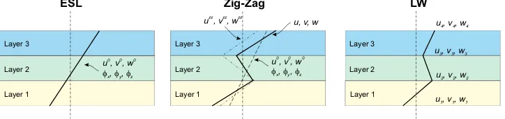
thickness by using a suitable assembly procedure. This leads to the so-called layer-wise (LW) theory [5, 11–17]. Each single layer can be modelled using classical plate theory, FSDT or HSDT. The displacement functions are cho-sen appropriately so that the continuity of displacements can be imposed at the interfaces during the assembly procedure. The change in the slope at the interfaces is routinely obtained by solving the problem. The assumed dis-placement field through the thickness for an LW theory is illustrated in Figure (2). It is evident that if LW theory is used, the displacement field is more
Layer 1 Layer 2 Layer 3
u , v , w1 1 1 u , v , w2 2 2 u , v , w3 3 3 u , v , w4 4 4
Layer 1 Layer 2 Layer 3
u , v , w , 0 0 0
fxf fy, z u , v , wzz zz zz
u, v, w
Layer 1 Layer 2 Layer 3
u , v , w , , 0 0 0
f f fx y z
[image:6.612.126.488.259.345.2]ESL Zig-Zag LW
Figure 2: Example of first order ESL, Zig-Zag and LW displacement distributions through
the thickness
especially for large orthotropic and thickness ratios. Even for thin plates with typical width to thickness ratio of 50, the error on the fundamental frequency can be as high as 10% [18–20] or 30% for multifield problems [12], and com-pletely wrong even by a order of magnitude for sandwich plates [17]. The need to use of a layer wise theory for obtaining accurate results cannot be overstated. Understandably the layer wise theory requires a large number of degrees of freedom which of course, depends on the number of layers. At present the problem is solved generally in exceptional circumstances by using the finite element method (FEM) [21] requiring a huge number of el-ements, thus embarking on an excessively large number of nodes to model the structure. This is probably the main reason why the layer wise the-ory is not favoured and often overlooked and, as an alternative, less accurate zig-zag theories are sought instead. Apparently the layer wise based finite ele-ments are mainly (if not solely) used for modelling delamination in ABAQUS software (called continuous shell elements) requiring large computational re-sources.
general boundary conditions, a dynamic stiffness matrix which contains all the natural frequencies of the element can be developed. This element for a plate has the shape of a strip that can be rotated and assembled to form a geometrically complex structure and yet the exactness of the solution can be retained. The results, in fact, will be mesh independent and with very few elements any number of required natural frequencies and mode shapes can be obtained to any desired accuracy for a structure that can be modelled or idealised as plate assemblies. The use of the DSM will allow an efficient use of LW theories because of the limited number of degrees of freedom required by the DSM unlike the FEM. The DSM has no limitation on the number of natural frequencies that can be computed. Thus it is significantly more computational efficient than the FEM.
The DSM has been largely developed for bars and beams [24–31] and im-plemented and validated in programs such as BUNVIS-RG [47] and PFVI-BAT [48].
shear deformation and rotatory inertia but their investigation was focused on isotropic plates [43]. In a parallel investigation, the authors also devel-oped the corresponding DSM for inplane free vibratory motion of isotropic plates [44] wherein a set of previously missed inplane modes was identified. Following these earlier investigations, the DSM was extended by the authors to composite plates using the first order shear deformation theory (FSDT) see [45,46] and Reddy’s high order shear deformation theory in [49]. Some ap-plication of the theory to aeronautical structures have been reported in [50]. These developments by the authors have been implemented in a computer program called DySAP.
In this paper, the extension of the DSM using a first order layer wise theory based on the CUF is presented, the results from the theory are validated and the superior accuracy is demonstrated. In Section (2) the fundamental equa-tions of solid mechanics relevant to the investigation are presented. Next, CUF is used to derive the equations of motion and boundary conditions for one orthotropic layer in explicit form in the first instance. In section (3), a novel method, called the L-matrix method has been presented to obtain au-tomatically the equations of motions and boundary condition of a plate with
the formulated problem is developed and the dynamic stiffness matrix of the element is obtained (section (4.1)). Assembly and boundary conditions are dealt with in sections (4.2) and (4.3) respectively. The Wittrick and Williams algorithm has been summarised in section (4.4) and an efficient procedure to obtain the mode shapes from as few as one element is presented in sec-tion (4.5). Given the complexity of the problem, a step by step procedure to obtain the DSM matrix for a layer wise formulation is given in section (5). In section (6), the developed formulation is first validate against Navier type solutions and then used to obtain closed form solution of multilayered composite plates with different boundary conditions which hitherto have not been obtained. These results can be used as benchmark for validating finite element and other approximate models. In the last section, some conclusions are drawn.
2. PRELIMINARIES: FROM PLATE MODEL TO GENERALISED
EQUATIONS OF MOTION BY THE CARRERA’S UNIFIED
FORMULATION (CUF)
The Carrera’s Unified Formulation (CUF) [12, 14, 16, 17, 22, 23] has been used in this section to obtain the equations of motion and boundary con-ditions for a multilayered plate. The prerequisites needed to formulate the problem in the CUF notation can be summarised as:
The above details are substituted into Hamilton’s principle to give a 3×3 matrix, often called the nucleus (section (2.4)), which can be conveniently expanded to the required plate theory depending on its order and assembled across the layers for composites to give either the FE stiffness matrix or the Navier’s type analytical stiffness matrix of the system [12, 14, 16, 17, 22, 23]. The CUF nucleus, different from previously published, has been used to obtain the differential equations of motion of the system in this paper (section (2.5)).
2.1. Displacement formulation
The displacement field is formulated by using thickness functionsFτ(z) in order to reduce the 3D problem where the unknown displacementsu(x, y, z, t) =
{u, v, w}are function ofx, y, z and tto a 2D problem for which the displace-ments are only function of 2 independent variables (x, y and t). By using the CUF, plate theories of any order (NCU F) can be formulated by using a unified notation.
uk(x, y, z, t) =Fb(z)ukb(x, y, t) +Fr(z)ukr(x, y, t) +Ft(z)ukt(x, y, t) (1) for r = 2, . . . , NCU F −1 where NCU F is the order of the plate theory to be used and the superscriptkrefer to the layer number. Eq.(1) can be rewritten in a more compact form by making use of Einstein’s notation where a double subscript stands for the usual summation
thickness function Fτ take the form of Legendre’s polynomials
Ft=
P0+P1
2 , Fb =
P0 −P1
2 , Fr =Pr−Pr−2 r= 2, . . . , N (3) where Pi(ζk) is the i-order Legendre polynomial in the domain−1≤ ζk ≤1 and ζk =z/hk. The first five Legendre polynomials are:
P0 = 1 P1 =ζk P2 = 3ζ2
k−1
2 P3 =
5ζ3 k−3ζk
2 P4 =
35ζ4
k −30ζk2+ 3 8
(4) The choice of these functions is not arbitrary but they must satisfy the fol-lowing fundamental properties:
ζk=
1 : Ft= 1, Fb = 0, Fr = 0
−1 : Ft= 0, Fb = 1, Fr = 0
(5)
which implies that. uk
t and ukb are in fact the displacements at the top and bottom of the kth layer (see Eq. (1)). This is important to ensure com-patibility at the interfaces between layers without the need to use Lagrange multipliers but by simply assembling the stiffness terms (or differential equa-tions) in the right order noting that:
ukt =u(bk+1), with k = 1, . . . , NL−1 (6)
2.2. Geometrical equations: strain-displacement relationships
The strain ε for the kth layer can written as εkT =h εxx, εyy, εzz, εyz, εxz, εxy
ik
=h ε1, ε2, ε3, ε4, ε5, ε6
ik
(7)
The above vector can be split into two, showing inplane strainεp = [εxx, εyy, εxy] and out of plane or normal strain εn = [εxz, εyz, εzz]. Their relation to the displacements u= [u, v, w] can be written as
where the differential or partial derivative matrices can be written as:
Dp =
∂x 0 0 0 ∂y 0
∂y ∂x 0
, Dnp =
0 0 ∂x 0 0 ∂y
0 0 0
, Dnz =
∂z 0 0 0 ∂z 0 0 0 ∂z
(9)
with ∂x=∂/∂x, ∂y =∂/∂y, ∂z =∂/∂z.
2.3. Constitutive equations: stress-strain relations
The complete 3D constitutive equations are used since thickness locking is generally not present for layer wise theories [51]. The stresses σk are
σkT =h σxx, σyy, σzz, σyz, σxz, σxy ik
=h σ1, σ2, σ3, σ4, σ5, σ6
ik
(10)
are related to the strain in the global reference system for orthotropic mate-rials by
σkp =Ckppεpk+Ckpnεkn , σkn=CkpnTεpk+Cknnεkn (11) where
Ckpp =
C11 C12 C16
C12 C22 C26
C16 C26 C66
k
Ckpn =
0 0 C13 0 0 C23 0 0 C36
k
Cknn =
C55 C45 0
C45 C44 0
0 0 C33
k (12)
σkTp = h σ1, σ2, σ6
ik
σkTn = h σ5, σ4, σ3
ik
(13)
εkTp = h ε1, ε2, ε6
ik
εkTn = h ε5, ε4, ε3
ik
(14)
2.4. Developing CUF nucleus K
Once the model and the governing equation have been formulated, Hamil-ton’s principle can now be used to obtain the equations of motion. The principle can be written by using the matrix form of the equations as
Nl
X
k=1
Z
Ak
Z
hk
n
δεkpGTσkpC +δεknGTσknCo dAk dz =δLe−δLin (15)
whereLinis the work done by the inertia forces andLeby the external forces. In order to obtain the fundamental nucleus the following substitution into Eq. (15) should be made:
(i) Constitutive relations Eq. (11) ; (ii) Geometric relations Eq. (8); (iii) Displacement formulation Eq. (2);
Finally by developing the matrix products and integrating by part equations of motion and natural boundary conditions are obtained. For the sake of brevity each single step is not reported here. The final result is a system of equations in matrix form so that
Kkτ s uks + Mkτ s u¨ks = 0 (16)
and the natural boundary conditions
ukτ = ¯ukτ or Πkτ sd uks = ¯Fkτ (17)
where τ ands are indexes which go from 1 to the order of the chosen formu-lation, i.e. the order of expansion of the displacement polynomials.
when properly assembled through the thickness for different layers, gives the equations of motion of the plate.
Kkτ s = Z
Ak
− DTpCkppDpIEτ s− DTpCkpnDnpIEτ s− DTpCkpnIEτ s,z
−DTnpCkTpnDpIEτ s−DTnpCknnDnpIEτ s−DTnpCknnIEτ s,z +CkTpnDpIEτ,zs+CknnDnpIEτ,zs+CknnIEτ,zs,z dz
(18)
The matrix Mkτ s is the mass matrix (shown below), which needs to be assembled across the layers just like the stiffness matrix Kkτ s.
Mkτ s = Z
Ak
ρkIEτ s dz (19)
The boundary conditions are formulated by 3×1 vector which needs to be assembled as well.
Πkτ s = Z
Ak
ITpCkppDpIEτ s+ITpCkpnDnpIEτ s+ITpCkpnIEτ s,z
+ITnpCkTpnDpIEτ s+ITnpCknnDnpIEτ s+ITnpCknnIEτ s,z dz (20)
achieve this, the following matrices are used:
I =
1 0 0 0 1 0 0 0 1
, Ip =
Γb 0 0
0 ΓL 0
ΓL Γb 0
,Inp =
0 0 Γb 0 0 ΓL
0 0 0
(21)
The integrals through the thickness are written as:
Eτ s= ∫ hk
FτFs dz Eτ,zs = ∫ hk
Fτ,zFs dz Eτ s,z = ∫
hk
FτFs,z dz Eτ,zs,z = ∫ hk
Fτ,zFs,z dz
(22)
Thus the explicit terms of the fundamental nucleus can be written as
Kkτ s
11 = (−C11k∂x2−2C16k∂x∂y−C66k∂y2)Eτ s+C55k Eτ,zs,z
Kkτ s
12 = (−C16k∂x2−(C12k +C66k)∂x∂y−C26k∂y2)Eτ s+C45kEτ,zs,z
Kkτ s
13 = (C55k∂x+C45k∂y)Eτ,zs−(C13k∂x+C36k∂y)Eτ s,z
Kkτ s
21 = (−C16k∂x2−(C12k +C66k)∂x∂y−C26k∂y2)Eτ s+C45kEτ,zs,z
Kkτ s
22 = (−C66k∂x2−2C26k∂x∂y−C22k∂y2)Eτ s+C44k Eτ,zs,z
Kkτ s
23 = (C45k∂x+C44k∂y)Eτ,zs−(C36k∂x+C23k∂y)Eτ s,z
Kkτ s
31 = (C13k∂x+C36k∂y)Eτ,zs−(C55k∂x+C45k∂y)Eτ s,z
Kkτ s
32 = (C36k∂x+C23k∂y)Eτ,zs−(C45k∂x+C44k∂y)Eτ s,z
Kkτ s
33 = (−C55k∂x2−2C45k∂x∂y−C44k∂y2)Eτ s+C33k Eτ,zs,z
(23)
Kkτ s
11 = Kkτ s22 = Kkτ s33 = ρk Eτ s
Kkτ s
and the boundary conditions are:
Πkτ s
11 = (∂x(ΓbC11k + ΓLC16k) +∂y(ΓbC16k + ΓLC66k))Eτ s Πkτ s
12 = (∂x(ΓbC16k + ΓLC66k) +∂y(ΓbC12k + ΓLC26k))Eτ s Πkτ s
13 = (ΓbC13k + ΓLC36k)Eτ s,z Πkτ s
21 = (∂x(ΓLC12k + ΓbC16k) +∂y(ΓLC26k + ΓbC66k))Eτ s Πkτ s
22 = (∂x(ΓLC26k + ΓbC66k) +∂y(ΓLC22k + ΓbC26k))Eτ s Πkτ s
23 = (ΓLC23k + ΓbC36k)Eτ s,z Πkτ s
31 = (ΓLC45k + ΓbC55k)Eτ s,z Πkτ s
32 = (ΓLC44k + ΓbC45k)Eτ s,z Πkτ s
33 = (∂x(ΓLC45k + ΓbC55k) +∂y(ΓLC44k + ΓbC45k))Eτ s
(25)
2.5. General equations of motion for first order layer wise plate theory, LD1
By using the CUF, any order of expansion, i.e. any higher order plate theory can be obtained by suitably expanding the indexes τ and s in Eq. (23). In this study, the expansion is limited to the first order and thus, the indexes τ and s will simply refer to the bottom b and top t interfaces of the kth layer. This formulation is usually refereed to in the literature as LD1 [12, 14, 16, 17, 22, 23]. The displacement functions, by referring to Eq. (1), can be written as
uk(x, y, z, t) =Fb(z)ukb(x, y, t) +Ft(z)ukt(x, y, t) (26) where the thickness functions (see Eq. (3)) can be written as
Ft = 1 2 −
z
h, Fb =
1 2+
z
h, (27)
and
ukb =
ukb, vbk, wkbT
, ukt =
ukt, vtk, wktT
Once the displacement formulation has been chosen as the one related to Eq. (26) and (27) the nuclei can obtained by using equations (18) and (23) by computing the integrals in Eq. (22). For the kth layer, the nucleus can be split into four 3×3 submarines which will be referred to as Kkbb, Kkbt, Kktb, Kktt. Also the mass matrix can be computed form Eq. (19) and (24) in the same way to give Mkbb,Mkbt,Mktb,Mktt.
Kkτ s uks + Mkτ s u¨ks = 0 (29)
Equation (29) can be written explicitly as 6 differential equations of motion. These 6 differential equations describe the behaviour of only 1 layer using a first order layer wise plate formulation called LD1.
+C55k
hk −13hk
Ck 11 ∂
2
∂x2 + 2C16k ∂ 2
∂x∂y +C66k ∂
2
∂y2
uk b
−Ck55
hk +16hk
Ck 11 ∂
2
∂x2 + 2C16k ∂
2
∂x∂y +C k 66 ∂ 2 ∂y2 uk t
+C45k
hk −13hk
Ck 16 ∂
2
∂x2 + (C12k +C66k ) ∂ 2
∂x∂y +C26k ∂
2
∂y2
vk b
−Ck45
hk +
1 6h
kCk 16 ∂
2
∂x2 + (C12k +C66k ) ∂
2
∂x∂y +C k 26∂ 2 ∂y2 vk t +1 2 (Ck
13−C55k)∂x∂ + (C k
36−C45k )∂y∂
wk b
−12(Ck
13+C55k)∂x∂ + (C k
36+C45k)∂y∂
wk t
+1 3h
kρk ∂2ukb
∂t2 +16hkρk ∂ 2uk
t
∂t2 = 0
(30)
+C45k
hk −13hk
Ck 16 ∂
2
∂x2 + (C12k +C66k ) ∂ 2
∂x∂y +C26k ∂
2
∂y2
uk b
−Ck45
hk +16hk
Ck 16 ∂
2
∂x2 + (C12k +C66k ) ∂
2
∂x∂y +C k 26∂ 2 ∂y2 uk t
+C44k
hk −13hk
Ck 66 ∂
2
∂x2 + 2C26k ∂ 2
∂x∂y +C22k ∂
2
∂y2
vk b
−Ck44
hk +
1 6h
kCk 66 ∂
2
∂x2 + 2C26k ∂
2
∂x∂y +C k 22 ∂ 2 ∂y2 vk t +1 2 (Ck
36−C45k)∂x∂ + (C k
23−C44k )∂y∂
wk b
−12(Ck
36+C45k)∂x∂ + (C k
23+C44k)∂y∂
wk t
+1 3h
kρk ∂2vkb
∂t2 +16hkρk ∂ 2vk
t
∂t2 = 0
+12(Ck
55−C13k)∂x∂ + (C45k −C36k)∂y∂
uk b
−12(Ck
55+C13k)∂x∂ + (C k
45+C36k)∂y∂ uk t +1 2 (Ck
45−C36k)∂x∂ + (C k
44−C23k)∂y∂
vk b
−12(Ck
45+C36k)∂x∂ + (C44k +C23k)∂y∂
vk t
+Ck33
hk − 13hk
Ck 55 ∂
2
∂x2 + 2C45k ∂
2
∂x∂y +C k 44∂ 2 ∂y2 wk b
−C33k
hk + 16hk
Ck 55 ∂
2
∂x2 + 2C45k ∂ 2
∂x∂y +C44k ∂
2
∂y2
wk t
+13hkρk ∂2wkb
∂t2 +
1 6h
kρk ∂2wkt
∂t2 = 0
(32)
−Ck55
hk +16hk
Ck 11 ∂
2
∂x2 + 2C16k ∂
2
∂x∂y +C k 66 ∂ 2 ∂y2 uk b
+C55k
hk −13hk
Ck 11 ∂
2
∂x2 + 2C16k ∂ 2
∂x∂y +C66k ∂
2
∂y2
uk t
−Ck45
hk +
1 6h
kCk 16 ∂
2
∂x2 + (C12k +C66k ) ∂
2
∂x∂y +C k 26∂ 2 ∂y2 vk b
+C45k
hk −16hk
Ck 16 ∂
2
∂x2 + (C12k +C66k ) ∂
2
∂x∂y +C k 26∂ 2 ∂y2 vk t
+12(Ck
13+C55k)∂x∂ + (C36k +C45k)∂y∂ wk b −1 2 (Ck
13−C55k)∂x∂ + (C k
36−C45k)∂y∂
wk t
+16hkρk ∂2ukb
∂t2 +13hkρk ∂ 2uk
t
∂t2 = 0
(33)
−Ck45
hk +16hk
Ck 16 ∂
2
∂x2 + (C12k +C66k ) ∂ 2
∂x∂y +C k 26∂ 2 ∂y2 uk b
+C45k
hk −13hk
Ck 16 ∂
2
∂x2 + (C12k +C66k ) ∂
2
∂x∂y +C k 26∂ 2 ∂y2 uk t
−Ck44
hk +16hk
Ck 66 ∂
2
∂x2 + 2C26k ∂ 2
∂x∂y +C22k ∂
2
∂y2
vk b
+C44k
hk −13hk
Ck 66 ∂
2
∂x2 + 2C26k ∂
2
∂x∂y +C k 22 ∂ 2 ∂y2 vk t
+12(C36k +C45k)∂x∂ + (C k
23+C44k)∂y∂
wbk
−12(Ck
36−C45k)∂x∂ + (C k
23−C44k)∂y∂
wk t
+1 6h
kρk ∂2vkb
∂t2 +13hkρk ∂ 2vk
t
∂t2 = 0
+12(Ck
55+C13k)∂x∂ + (C45k +C36k)∂y∂
uk b
−12(Ck
55−C13k)∂x∂ + (C k
45−C36k)∂y∂ uk t +1 2 (Ck
45+C36k)∂x∂ + (C k
44+C23k)∂y∂
vk b
−12(Ck
45−C36k)∂x∂ + (C44k −C23k)∂y∂
vk t
−C33k
hk + 16hk
Ck 55 ∂
2
∂x2 + 2C45k ∂
2
∂x∂y +C k 44∂ 2 ∂y2 wk b
+Ck33
hk − 13hk
Ck 55 ∂
2
∂x2 + 2C45k ∂ 2
∂x∂y +C44k ∂
2
∂y2
wk t
+16hkρk ∂2wkb
∂t2 +
1 3h
kρk ∂2wkt
∂t2 = 0
(35)
and the boundary condition can be written explicitly by using Eqs. (20) and (25) and putting ΓL = 0 and Γb = 1 to limit our focus to the sides at x= 0 and x=b.
Fub = +
1 3hk
Ck
11∂x∂ +C16k ∂y∂
uk
b +16hk
Ck
11∂x∂ +C16k ∂y∂
uk t
+13hkCk
16∂x∂ +C k 12∂y∂
vk b +16h
kCk
16∂x∂ +C k 12∂y∂
vk t
−C13k
2 w k b + Ck 13 2 w k t (36)
Fvb = +
1 3hk
Ck
16∂x∂ +C66k ∂y∂
uk
b +16hk
Ck
16∂x∂ +C66k ∂y∂
uk t
+1 3h
kCk
66∂x∂ +C k 26∂y∂
vk b +16h
kCk
66∂x∂ +C k 26∂y∂
vk t
−C36k
2 wbk + Ck
36
2 wkt
(37)
Fwb = −
Ck
55
2 ukb + Ck
55
2 ukt − Ck
45
2 vkb + Ck
45
2 vkt +1
3h kCk
55∂x∂ +C k 45∂y∂
wb k+16hk
Ck
55∂x∂ +C k 45∂y∂
wk t
(38)
Fub = +
1 6hk
Ck
11∂x∂ +C16k ∂y∂
uk
b +13hk
Ck
11∂x∂ +C16k ∂y∂
uk t
+16hkCk
16∂x∂ +C k 12∂y∂
vk b +13h
kCk
16∂x∂ +C k 12∂y∂
vk t
−C13k
Fvb = +
1 6hk
Ck
16∂x∂ +C66k ∂y∂
uk
b +13hk
Ck
16∂x∂ +C66k ∂y∂
uk t
+16hkCk
66∂x∂ +C k 26∂y∂
vk b +13h
kCk
66∂x∂ +C k 26∂y∂
vk t
−C36k
2 w k
b +
Ck
36
2 w k t
(40)
Fwb = −
Ck
55
2 u k b +
Ck
55
2 u k
t −
Ck
45
2 v k b +
Ck
45
2 v k t
+16hkCk
55∂x∂ +C k 45∂y∂
wk b +13h
kCk
55∂x∂ +C k 45∂y∂
wk t
(41)
Sign convention for forces and displacements are shown in Figure (3). The above system of quadratic, fully coupled, constant coefficient partial differential equations needs to be solved simultaneously along with the BC to obtain the solution for 1 layer.
Figure 3: Coordinate system and notations for displacements and forces for a multilayered
plate.
2.6. From partial to ordinary differential equations for plates with two
oppo-site sides simply supported
The system of partial differential equations for 1 layer can be reduced to a set of ordinary ones (one for each m) by making use of sinwaves in the y
direction and the exponential function for the time t. Thus
uk
b(x, y, t) = ∞
X
m=1
Uk
b(x)sin(αmy)eiωt;ukt(x, y, t) = ∞
X
m=1
Uk
t(x)sin(αmy)eiωt
vbk(x, y, t) = ∞
X
m=1
Vbk(x)cos(αmy)eiωt; vtk(x, y, t) = ∞
X
m=1
Vtk(x)cos(αmy)eiωt
wkb(x, y, t) = ∞
X
m=1
Wbk(x)sin(αmy)eiωt; wtk(x, y, t) = ∞
X
m=1
Wtk(x)sin(αmy)eiωt (42)
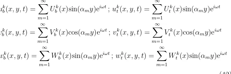
where ω is an arbitrary circular or angular frequency, αm = mπL and m = 1,2, . . . ,∞. This is also refereed to in the literature as Levy’s solution and complies with the boundary condition associated to a plate where the two sides a y=0 and y=L are simply supported (SS) (i.e. uk
assuming to study a material for which, Ck
16 = C26k = C36k = C45k = 01 (i.e. either 0 or 90 degree ply for composite plates) the following system of fully coupled, quadratic, ordinary differential equations can be written as
a1+3Ck
55)
3hk Ub+
a1−6Ck
55
6hk Ut+
a2
3hkV
0
b+6a2hkV
0
t +6a3hkW
0
b+6a4hkW
0
t−13Ck11hkU
00
b −16C11khkU
00
t = 0
−2a5−6C
k
44)
6hk Vb−a5+6C
k
44
6hk Vt+
a7
6hkWb+6a6hkWt−
a2
3hkU
0
b− a2
6hkU
0
t−13C66khkV
00
b −16C66khkV
00
t = 0 a7
6hkVb− a6
6hkVt−
2a8−6Ck
33
6hk Wb−a8+6C
k
33
6hk Wt−
a3
6hkU
0
b+ a4
6hkU
0
t−13C55khkWb00−16C55khkWt00 = 0 a1−6Ck
55)
3hk Ub+a1+3C
k
55
6hk Ut+
a2
6hkV
0
b+ a2
3hkV
0
t −6a4hkW
0
b− a3
6hkW
0
t−16Ck11hkUb00−13C11khkUt00 = 0
−a5+6C
k
44)
6hk Vb−2a5−6C
k
44
6hk Vt−
a6
6hkWb− a7
6hkWt−
a2
6hkU
0
b− a2
3hkU
0
t−16C66khkVb00−13C66khkVt00 = 0 a6
6hkVb− a7
6hkVt−
a8+6Ck
33
6hk Wb−2a8−6C
k
33
6hk Wt−
a4
6hkU
0
b+ a3
6hkU
0
t−16C55khkW
00
b −13C55khkW
00
t = 0
(43) where the prime or upper suffix 0
denotes the ordinary derivative d/dx and
ak
1 = hk 2
(α2
mC66k −ω2ρk) , ak2 = αmhk2(C12k +C66k)
ak
3 = 3hk(C13k −C55k) , a4k = −3hk(C13k +C55k)
ak
5 = hk 2
(ω2ρ
k−α2mC22k) , ak6 = −3αmhk(C23k +C44k)
ak
7 = 3αmhk(C23k −C44k) , ak8 = 2hk 2
(ω2ρ
k−α2mC44k)
(44)
and the boundary conditions are Fk
U b = −16αmh kCk
12(2Vbk+Vtk)− 12C k
13(Wbk−Wtk) + 16C k
11hk(2U 0k b +U
0k t )
Fk
V b = +16αmh kCk
66(2Ubk+Utk) + 16C k 66hk(2V
0k b +V
0k t )
Fk
W b = −12C k
55(Ubk−Utk) + 16C k
55hk(2W 0k b +W
0k t )
FU tk = −16αmhkC12k(Vbk+ 2Vtk)− 12C k
13(Wbk−Wtk) + 16C k 11hk(U
0k b + 2U
0k t )
Fk
V t = +16αmh kCk
66(Ubk+ 2Utk) + 16C k 66hk(V
0k b + 2V
0k t )
FW tk = −12C55k(Ubk−Utk) + 16C k 55hk(W
0k b + 2W
0k t )
(45)
1This is a necessary condition in order for the trigonometric function to be a solution
3. THE L-MATRIX METHOD
3.1. Use of the L matrix for systematic generation of the equations for N
layers
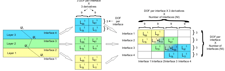
The above equations are valid for only one layer. If more than one layer is used, the fundamental CUF nucleus K (Eq. (18)) should be assembled across the new number of layers and the new equations of motion which will be coupled (layer by layer) should be developed all over again. For this reason a way of assembling directly the differential equations of motion and boundary conditions starting sequentially from layer 1 (Eqs. (43) and (45)) has been devised. This method hereafter is referred to as the L-matrix method. The method can find its applications in a multitude of problems where the number of differential equations to solve changes from one case to the other due to external factors (such as number of layers, order of the displacement models, etc...). It is inconvenient to rewrite the equations and solve the system for each case. This method uses a matrixLto represent the system of differential equations. The matrix L has a number of rows equal to the number of differential equations. In the present case, the number is 6 because Uk
b = [Ubk, Vbk, Wbk] and Utk = [Utk, Vtk, Wtk]. The number of columns is equal to the number of unknowns 6 in this case (Uk
b = [Ubk, Vbk, Wbk] and
Uk
t = [Utk, Vtk, Wtk]) times the number of derivative orders which is 3, namely derivative 0, first order and second order for a total of 18 columns for 1 layer. The Lmatrix can be split into 4 sub-matrices which will refer to the bottom layer, and top layer of each ply. e.g. the kth ply.
form as Lk BB L k BT Lk
T B L
k T T ˜ Uk B ˜ Uk T = 0 0 (46) where ˜
UBk = [UBk, U0k B, U
00k B , VBk, V
0k B , V
00k
B , WBk, W 0k B, W
00k B ]T
˜
UTk = [UTk, U0k T , U
00k T , VTk, V
0k T , V
00k
T , WTk, W 0k T , W
00k T ]T
(47)
and
LkB B= ak
1+3C
k
55
3hk 0 −
Ck
11hk
3 0
ak
2
3hk 0 0
ak
3
6hk 0
0 −a
k
2
3hk 0 −
ak
5−3C
k
44
3hk 0 −
Ck
66hk
3
ak
7
6hk 0 0
0 −a
k
3
6hk 0
ak
7
6hk 0 0 −
ak
8−3C
k
33
3hk 0 −
Ck 55hk 3 (48)
LkB T =
ak1−6C
k
55
6hk 0 −
C11hk k
6 0
ak2
6hk 0 0
ak4
6hk 0
0 −a
k
2
6hk 0 −
ak5+6C
k
44
6hk 0 −
C66hk k
6
ak6
6hk 0 0
0 a
k
4
6hk 0 −
ak
6
6hk 0 0 −
ak
8+6C
k
33
6hk 0 −
Ck 55hk 6 (49)
LkT B = ak
1−6C
k
55
6hk 0 −
Ck
11hk
6 0
ak
2
6hk 0 0 −
ak
4
6hk 0
0 −a
k
2
6hk 0 −
ak
5+6C
k
44
6hk 0 −
Ck
66hk
6 −
ak
6
6hk 0 0
0 −a
k
4
6hk 0
ak
6
6hk 0 0 −
ak
8+6C
k
33
6hk 0 −
Ck 55hk 6 (50)
LkB B =
ak1+3C
k
55
3hk 0 −
C11hk k
3 0
ak2
3hk 0 0 −
ak3
6hk 0
0 −a
k
2
3hk 0 −
ak
5−3C
k
44
3hk 0 −
Ck
66hk
3 −
ak
7
6hk 0 0
0 a
k
3
6hk 0 −
ak
7
6hk 0 0 −
ak
8−3C
k
33
3hk 0 −
Layer 1 Layer 2 Layer 3 LBB 3 LTT 3 LTB 3 LBT 3 Interface 1 Interface 4 Interface 3 Interface 2 LBB 2 LTT 2 LTB 2 LBT 2 LBB 1 LTT 1 LTB 1 LBT 1 U 4 U3 U2 U1 } }
}
}
9 3 3 9 3 DOF per interfaceX 3 derivatives DOF per interface LBB 1
L +TT 1 LTT 2 LTB 1 LBT 1 Interface 1 Interface 2 Interface 3 Interface 4 }3 }3 }3 }3
}
DOF per interface
X Number of Interfaces (NI) L +TT
2 LBB 3 LTT 3 LTB 3 LBT 3 LBT 2 LTB 2
Interface 1 Interface 2Interface 3 Interface 4
}
9 9
}
9}
}
9}
DOF per interface X 3 derivatives [image:26.612.105.554.78.220.2]X Number of Interfaces (NI)
Figure 4: Schematic of how to assemble theLmatrices for each layer to obtain the global
L, i.e. the global system of differential equations
The global system of second order differential equations can be written then by using the global matrix Lin the following form
L1 BB L 1
BT 0 . . . 0
L1
T B L
1
T T +L
2
BB L
2
BT . . . 0
0 L2
T B L
2
T T . . . 0
... ... ... . .. ...
0 0 0 . . . LNlT T
˜ U1 ˜ U2 ˜ U3 ... ˜ UNI = 0 0 0 ... 0 (52) or,
LU˜ =0 (53)
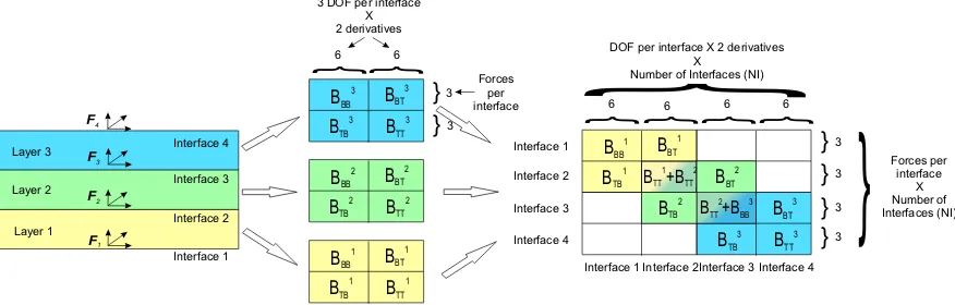
The boundary conditions in Eq. (45) can also be written in matrix form as Fk B Fk T = Bk BB B k BT Bk
T B B
k T T ˆ Uk B ˆ Uk T (54) where ˆ Uk
B= [U
k B, U
0k B, VBk, V
0k
B, WBk, W 0k B]T
ˆ
Uk
T = [U
k T, U
0k T , VTk, V
0k
T , WTk, W 0k T ]T
(55)
and
BkB B = 0 C k 11hk 3 −
αmC k
12hk
3 0 −
C13hk k
2 0
αmCk66hk
3 0 0
Ck
66hk
3 0 0
−C
k
55hk
2 0 0 0 0
Ck 55hk 3 (56)
BB Tk = 0 C k 11hk 6 −
αmC12hk k
6 0
Ck
13hk
2 0
αmC66hk k
6 0 0
Ck
66hk
6 0 0
Ck
55hk
2 0 0 0 0
Ck 55hk 6 (57) Bk T B =
0 C k 11hk 6 −
αmC12hk k
6 0 −
Ck
13hk
2 0
αmC66hk k
6 0 0
Ck
66hk
6 0 0
−C
k
55hk
2 0 0 0 0
Ck 55hk 6 (58)
BkT T = 0 C k 11hk 3 −
αmCk12hk
3 0
Ck
13hk
2 0
αmCk66hk
3 0 0
Ck
66hk
3 0 0
Ck
55hk
2 0 0 0 0
Ck 55hk 3 (59)
Layer 1 Layer 2 Layer 3 BBB 3 BTT 3 BTB 3 BBT 3 Interface 1 Interface 4 Interface 3 Interface 2 BBB 2 BTT 2 BTB 2 BBT 2 BBB 1 BTT 1 BTB 1 BBT 1 F4 F 3 F2 F1 } }
}
}
6 3 3 6 3 DOF per interfaceX 2 derivatives Forces per interface BBB 1
B +TT 1 BTT 2 BTB 1 BBT 1 Interface 1 Interface 2 Interface 3 Interface 4 }3 }3 }3 }3
}
Forces per interface
X Number of Interfaces (NI)
B +TT 2 BBB 3 BTT 3 BTB 3 BBT 3 BBT 2 BTB 2
Interface 1 Interface 2Interface 3 Interface 4
}
6 6
}
6}
}
6}
DOF per interface X 2 derivatives [image:28.612.113.551.78.218.2]X Number of Interfaces (NI)
Figure 5: Schematic of how to assemble theBmatrices for each layer to obtain the global
B, i.e. the global equations of the boundary conditions
F1 F2 F3 ... FNI = B1 BB B 1
BT 0 . . . 0
B1
T B B
1
T T +B
2
BB B
2
BT . . . 0
0 B2
T B B
2
T T . . . 0
... ... ... . .. ...
0 0 0 . . . BT TNl
ˆ U1 ˆ U2 ˆ U3 ... ˆ UNI (60) or,
F =BUˆ (61)
where rows of the global B are equal to the number of forces per interface which is equal to the number of displacements per interface (DOF = 3, i.e.
Fk
3.2. Solution of the differential equations with the L matrix method
The procedure to solve a system of ordinary differential equation of the second order with constant coefficients is given in (APPENDIX B). Once the matrix S˜ (see Eq. (B.3)) is known, the matrix S (see Eq. (B.7)) can then be consequently obtained via a change of variables . As explained in (APPENDIX B) a change of variable to reduce the second order system to a first order system is sought in the following form:
Z = [Z1, Z2, . . . , ZN]T =Uˆ = = [U1, U
0 1, V1, V
0
1, W1, W 0 1, U2, U
0 2, V2, V
0
2, W2, W 0
2, . . . , V 0
N I, WN I, W 0 N I]T
(62)
whereN = 3×N I×2 is the dimension of the unknown vector as well as the number of differential equations.
The main task now is to find an algorithm to transform the assembledL(Eq. (53)) matrix into the matrix S. In fact, by looking at Eq. (B.2) it could be˜ seen that only second derivatives should be on the left hand side (LHS) of the differential equations while, by looking at Eq. (43) for layer 1 and then looking at the system of equations written in compact form forNllayers (see Eq. (53)). Thus for each equations more than one second derivative appears. In order to obtain the matrixSfrom the globalLmatrix decoupling between the second derivatives is necessary and should be done row by row and only one second derivative should appear in each row. In this context the matrix L is devised so that every third column shows the value of the coefficient of a second derivative which makes decoupling of the second derivatives easier. In fact, in order to decouple the equations, these coefficients should be: (i)
column N and zero for column 3,6,9, . . . , N −3.
Once this is achieved, only one second derivative appears in each row and by setting the value of the coefficient to −1, is equivalent to moving that term on the LHS of the equation so that if these columns are removed from the transformed L, which is calledL, only the right hand side of the equation isˆ left, that is the matrix of the coefficient of the differential equations called
˜
S from which S can be obtained by adding rows with 0’s and 1’s to include the change of variables (see (APPENDIX B), Eq. (B.3) and (B.7)). The algorithm to transform the Lto theS˜is named by the authors forward and backward partial Gauss elimination (FBPGE) and is explained in details in (APPENDIX C).
Once the matrix S˜ (Eq. (B.3)) is obtained, and subsequently transformed to S (B.7), by following the procedure (explained in detail in (APPENDIX B)) the solution can be written in matrix form as:
Z1
Z2 ...
ZN
=
δ11 δ21 . . . δN1
δ12 δ22 . . . δN2 ... ... ... ...
δ1N δ2N . . . δN N
C1eλ1x
C2eλ2x ...
CNeλNx
(63)
where λi is the ith eigenvalue of the S matrix, δij is the jth element of the
ith eigenvector and C
i are the integration constants which needs to be deter-mined by using the boundary conditions.
The above equation can be written in matrix form as:
Z =δCeλx (64)
computing the boundary conditions. If only the displacements are needed, by remembering Eq. (62) only the rows 1,3,5, . . . , N should be taken, giving a solution in the following form:
U1(x) = C1δ11eλ1x+C2δ21eλ2x+. . .+CNδN1eλNx
V1(x) = C1δ13eλ1x+C2δ23eλ2x+. . .+CNδN3eλNx
W1(x) = C1δ15eλ1x+C2δ25eλ2x+. . .+CNδN5eλNx ...
WN I(x) = C1δ1(N−1)eλ1x+C2δ2(N−1)eλ2x+. . .+CNδN(N−1)eλNx
(65)
Once the displacements and their first derivatives are known, the boundary conditions can be easily obtained by recalling that the global Uˆ is equal to Z (Eq. (62)) and by substituting the solution (Eq. (64)) into the boundary conditions (Eq. (61)). This leads to
F =BδCeλx=ΛCeλx (66)
where the matrixΛcontains the coefficients for the calculating the boundary conditions and has dimensions (3 DOF × NI) × (N) where N is equal to 3 DOF × NI × 2 derivatives. The boundary conditions can be written in explicit form as
FU1(x) = C1Λ11e
λ1x+C
2Λ12eλ2x+. . .+CNΛ1NeλNx
FV1(x) = C1Λ21e
λ1x+C
2Λ22eλ2x+. . .+CNΛ2NeλNx
FW1(x) = C1Λ31e
λ1x+C
2Λ32eλ2x+. . .+CNΛ2NeλNx ...
FWN I(x) = C1Λ(N/2)1e
λ1x+C
2Λ(N/2)2eλ2x+. . .+CNΛ(N/2)NeλNx
Although resorting to the L matrix seems extremely convoluted and compli-cated, it is in fact the simplest way to solve a problem of such complex nature. The matrixLis simply a different way to write the differential equations for one layer. The greatest advantage is that it allows an automatic assembly of the differential equations for different layers (and if needed for different plate theories with increasing orders). In contrast to the structural problems in the literature, where by using a Navier type solution, the system becomes algebraic, or by using Levy’s solution the equations are written for one config-uration and then solved, by usingLmatrix method the differential equations can be written automatically, thus allowing the solution of the problem for any number of layer in an automatic way. Earlier attempts to assemble di-rectly the S matrix instead of using the L-matrix method failed due to the fact that more than one second derivative appears in each equation and then decoupling on the second derivatives was needed. This decoupling, physi-cally, represents the connection between each and every interface through the thickness and not only for the adjacent one but also for the subsequent ones. In fact, after decoupling of the second derivatives, unknowns coming from all the interfaces appear in each equation.
4. DYNAMIC STIFFNESS FORMULATION
4.1. Dynamic stiffness matrix
scenarios (i) free boundary: forces equal zero at x = 0 and x = b; (ii) clamped boundary: displacements equal zero atx= 0 andx=b; (iii) simply supported: a combination of displacements and forces equal to zero at x= 0 and x=b. A limitation to the classical method is that it can only be applied to study simple individual plates. By contrast, the solution obtained thus far, can be used to obtain the dynamic stiffness matrix of an element (similar to spectral elements [54]) which can be assembled to obtain the closed form exact results for geometrically more complex structures.
The procedure to obtain the DS matrix for any structural element can be summarised as:
(i) Seek a closed form solution of the governing differential equations of motion for a structural element in free vibration.
(ii) Apply a number of general boundary conditions equal to twice the number of integration constants in algebraic form; these are usually nodal displacements and forces.
(iii) Eliminate the constants by relating the harmonically varying nodal forces to the corresponding displacements which generates the frequency dependent dynamic stiffness matrix connecting the nodal forces to the nodal displacements.
The procedure to obtain closed form solution has already been explained in the previous section. This should now be followed by the imposition of generic boundary conditions on each interface for displacements and forces (see Fig. (6)).
write:
At x= 0 :
U1(0) =−U11, V1(0) =−V11, W1(0) =−W11
U2(0) =−U12, V2(0) =−V12, W2(0) =−W12 ...
UN I(0) =−U1N I, VN I(0) =−V1N I, WN I(0) = −W1N I
(68)
At x=b :
U1(b) =U21, V1(b) = V21, W1(b) =W21
U2(b) =U22, V2(b) = V22, W2(b) =W22 ...
UN I(b) = U2N I, VN I(b) =V2N I, WN I(b) =W2N I
(69)
By formulating Eqs. (65) for x = 0 and x= b and applying the BC in Eqs. (68) and (69), the following matrix relation for the nodal displacements is obtained:
U11
V11
W11
.. .
W1N I
U21
V21
W21
.. .
W2N I
=
−δ11 −δ21 . . . −δN1
−δ13 −δ23 . . . −δN3
−δ15 −δ25 . . . −δN5
..
. ... . .. ...
−δ1(N−1) −δ2(N−1) . . . −δN(N−1)
δ11eλ1b δ21eλ2b . . . δN1eλNb
δ13eλ1b δ23eλ2b . . . δN3eλNb
δ15eλ1b δ25eλ2b . . . δN5eλN b
..
. ... . .. ...
δ1(N−1)e
λ1b δ
2(N−1)e
λ2b . . . δ
N(N−1)e
λNb
C1 C2 C3 .. .
CN/2
CN/2+1
CN/2+2
CN/2+3
The above equation can be written in more compact form as
U =AC (71)
Also for the forces, general nodal forces are used as boundary conditions (see Fig. (6)):
At x= 0 :
FU1(0) =−F1U1, FV1(0) =−F1V1, FW1(0) =−F1W1
FU2(0) =−F1U2, FV2(0) =−F1V2, FW2(0) =−F1W2
...
FUN I(0) =−F1UN I, FVN I(0) =−F1VN I, FWN I(0) =−F1WN I
(72)
At x=b :
FU1(b) =F2U1, FV1(b) =F2V1, FW1(b) =F2W1
FU2(b) =F2U2, FV2(b) =F2V2, FW2(b) =F2W2
...
FUN I(b) = F2UN I, FVN I(b) = F2VN I, FWN I(b) =F2WN I
(73)
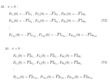
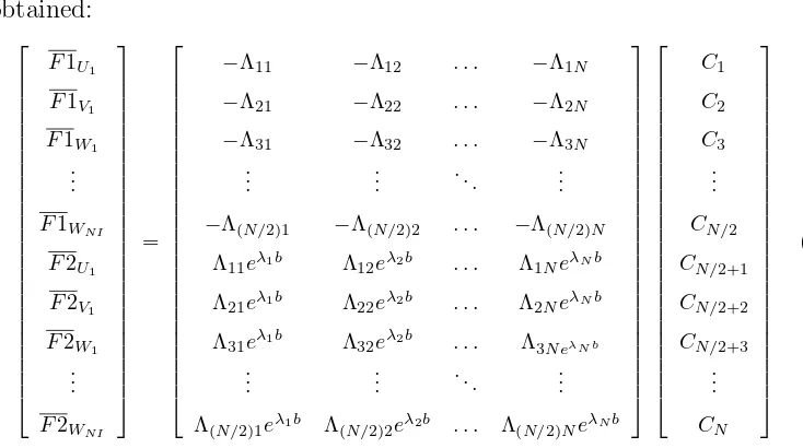
[image:35.612.123.509.181.460.2]obtained:
F1U1
F1V1
F1W1
.. .
F1WN I
F2U1
F2V1
F2W1
.. .
F2WN I
=
−Λ11 −Λ12 . . . −Λ1N −Λ21 −Λ22 . . . −Λ2N −Λ31 −Λ32 . . . −Λ3N
..
. ... . .. ...
−Λ(N/2)1 −Λ(N/2)2 . . . −Λ(N/2)N
Λ11eλ1b Λ12eλ2b . . . Λ1NeλNb
Λ21eλ1b Λ22eλ2b . . . Λ2NeλNb
Λ31eλ1b Λ32eλ2b . . . Λ3N eλN b
..
. ... . .. ...
Λ(N/2)1eλ1b Λ(N/2)2eλ2b . . . Λ(N/2)NeλNb
C1 C2 C3 .. .
CN/2
CN/2+1
CN/2+2
CN/2+3
.. . CN (74)
The above equation can be written in more compact for as
F =RC (75)
Layer 1 Layer 2 Interface 1 Interface NI Interface 3 Interface 2
U11V1 W1
F1 F1 F1
1 1 U1 V1 W1
U12V1 W1
F1 F1 F1
2 2 U2 V2 W2
U13V1 W1
F1 F1 F1
3 3 U3 V3 W3
U1NIV1 W1
F1 F1 F1
NI NI UNI VNI WNI
Line node 1
Line node 2
U21V2 W2
F2 F2 F2
1 1 U1 V1 W1
U22V2 W2
F2 F2 F2
2 2 U2 V2 W2
U23V2 W2
F2 F2 F2
3 3 U3 V3 W3
x y z
SS side
SS side
U2NIV2 W2
F2 F2 F2
NI NI UNI VNI WNI
[image:36.612.116.483.80.285.2]U1 V1 W1 F1U F1V F1W U2 V2 W2 F2U F2V F2W
The constant vector C from Eqs. (71) and (75) can now be eliminated to give the dynamic stiffness matrix of one element:
F =KU (76)
where
K =RA−1
(77)
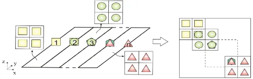
4.2. Assembly of the DS elements
[image:37.612.180.430.447.526.2]The dynamic stiffness matrix given by Eqs. (77) is the basic building block to compute the exact natural frequencies and mode shapes of a plate which is simply supported on at least two of their opposite sides and for such individual plate problems no coordinate transformation or offset connections are needed. As the DSM has many of the general features of the FEM, it has thus the capability to assemble element stiffness matrices to form the overall dynamic stiffness matrix of complex structures consisting of plate elements (see Figure (7)). For instance, plates with stringers connected at any arbitrary orientations can be analysed and yet exact results can be achieved.
Figure 7: Assembly of dynamic stiffness matrices
The global dynamic stiffness matrix can be written as
whereKGis a square matrix of dimensions: DOF×NI×NN (total number
of nodes in the structure).
4.3. Boundary conditions
The boundary conditions can be applied by using the well-known penalty method (often used in the FEM) or by simply removing rows and columns of the dynamic stiffness matrix corresponding to the degrees of freedom which need to be constrained. Due to the presence of degrees of freedom at each in-terface (see Figure (6)), a multitude of boundary condition can be applied at the required line nodes. A choice on whether or not to constrain the interface nodes at the boundaries has also to be addressed. As a matter of fact, layer wise plate models allow for constrains to be applied through the thickness differently from classical plate theories, having a quasi-3D representation. Although there are multiple possibilities, the implemented constrain types the associated degrees of freedom that are penalised are:
• Free end (F): no penalty
• Clamped end (C): penalty applied to Uk, Vk, Wk at each and every interface
• Simply supported (S): penalty applied to Vk, Wk at each and every interface thought the thickness
4.4. The Wittrick-Williams algorithm
[55] is recognisably the best available solution technique at present. The algorithm can be briefly summarised in the following steps:
(i) A trial frequencyω∗
is chosen to compute the dynamic stiffness matrix
K∗
of the final structure; (ii) K∗
is reduced to its upper triangular form by Gauss elimination to obtain K∗4
and the number of negative terms on the leading diago-nal of K∗4
is counted; this is known as the sign count s(K∗
) of the triangulated matrix;
(iii) The number (j) of natural frequencies (ω) of the structure which lie below the trial frequency (ω∗
) is then given by:
j =j0+s(K ∗
) (79)
wherej0 is the number of natural frequencies of all individual elements with clamped-clamped (C-C) boundary conditions on their opposite sides which still lie below the trial frequency ω∗
.
Assuming thatj0 is known, ands(K∗) can be obtained by counting the num-ber of negative terms in the diagonal of K∗4
, a suitable procedure can be devised, for example the bi-section method, to bracket any natural frequency between an upper and lower bound of the trial frequency ω∗
to any desired accuracy.
C-C frequency of the largest element in the global structure by running a sub-analysis. The largest element has also the lower C-C frequency of the whole structure. This frequency can be called omega limit ω∗
L and its limits the trial omega for whichj0 = 0. Thus, if the trial omega exceeds the omega limit, the structure is split automatically into smaller elements, for which, the new omega limit will be higher, and in this way additional frequencies can be computed.
4.5. Mode shape computation
Once natural frequencies have been computed, by using the global dy-namic stiffness matrix of Eq. (78) and a random force vector FG, the nodal
displacements corresponding to the given natural frequencies can be com-puted. So far, in the literature, the nodal displacements UGare used to plot
the mode shapes [24–39, 43–46]. In order to have a detailed plot, a large number of elements is required. In fact, this is not necessary in DSM. A new procedure to obtain the modal displacement as a function ofx, y, z has been devised and can be summarised in the following steps.
(i) The global nodal displacementUGis split into the element by element
displacement vector to giveU. A cycle on the elements will be needed. The ith element is analysed in the following steps.
(ii) By using the nodal displacementsU the integration constantsC of the element can be computed by using Eq. (71).
(iii) By using Eq. (65), the unknown displacements can be computed as a function of x.
(v) By using Eqs. (26) and (27) the 3D plot of the required mode and required element can be visualised.
By following the above procedure, with only 1 element, the exact mode shapes can be obtained.
5. SUMMARY OF THE DSM FORMULATION FOR A LAYER
WISE MODEL
Due to the complicated and convoluted steps required for developing this advanced dynamic stiffness element, a summary of the required steps is pre-sented below.
(i) Calculate theL (Eq. (46)) and B (Eq. (54)) matrices for each layer (ii) Assemble theLmatrix andBmatrix across the thickness layer by layer
as explained in Figure (4) and (5) and Eqs. (52) and (60)
(iii) Apply FBPGE (see (APPENDIX C)) to obtain the matrixS˜and then transform it to reduce the order (see (APPENDIX B)) to obtainS (Eq. (B.7))
(iv) Solve the reduced order system of differential equations to obtain the displacements and boundary conditions (integration constants are still unknown), i.e. calculate δ and λ to find the displacements (Eq. (64)) and Λ to find the boundary conditions (Eq. (66))
(v) Calculate the matrixA(Eq. (70)) for the displacements and the matrix R (Eq. (74)) for the forces
(vi) Calculate the DS matrix of the single multilayered element as K = A−1
(vii) Once the DS matrix of the single element is obtained, it is then pos-sible to rotate and assemble the elements to study complex structures (section (4.2))
(viii) Apply the required boundary conditions to the global structure (section (4.3))
(ix) Solve the matrix by using the classical Wittrick and Williams algorithm (section (4.4)) to calculate the natural frequencies
(x) Compute the mode shapes (section (4.5))
By following the above procedure, closed form analytical results for structures which can modelled as strip assemblies can be obtained by conducting a layer-wise analysis which increases the accuracy of result very considerably. The proposed method allows the investigation of sandwich plates with various interfaces, and can be used for modelling even delamination which is indeed a very difficult problem.
6. RESULTS
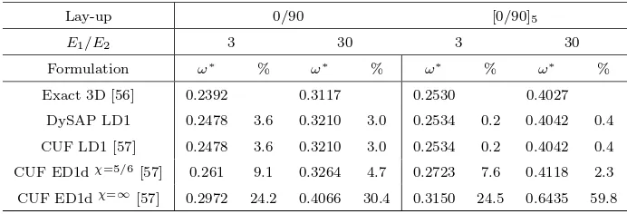
The plate studied has a side over thickness ratio a/h of 5 and has a square geometry. The material properties are as follow: G12/E2 = G13/E2 = 0.5,
G23/E2 = 0.35, ν12 =ν13= 0.3,ν23 = 0.49. Four different staking sequences are investigated: two skew-symmetric [0/90] and [0/90]5 and two symmetric [0/90/90/0] and [0/90/0/90/0]S. The total thickness of the 0 degree layers is equal to the total thickness of the 90 degree layers for all the configurations. Furthermore, 2 stiffness ratios are used, namely E1/E2 = 3 andE1/E2 = 30. The frequencies are given in non-dimensional form as ω∗
=ωhpρ/E2.
6.1. Validation and assessment for simply supported plates
Tables (1) and (2) show the results obtained for a plate simply sup-ported on all its four sides (SSSS) by using the new dynamic stiffness ele-ment (DySAP LD1). They are compared with Navier type solutions based on different plate theories such has CUF LD1, CUF ED1d χ=5/6, and CUF ED1dχ=∞
. In the table, LD1 refers to a first order layer wise theory which is equivalent to the one implemented in the paper, ED1d χ=5/6 refers to a first order equivalent single layer theory with a shear correction factor ofχ= 5/6, and ED1d χ=∞
from isotropic plates where the total thickness compared to the side length would define if a plate is “thin” or “thick”, for composite plates, the thick-ness of the single ply is more important than the total thickthick-ness of the plate. For thicker plies, higher order theories should be used not to compromise the accuracy of results. Furthermore, the level of anisotropy, which can be defined by the stiffness ratio E1/E2, also influences the accuracy of the re-sults. Plates with higher stiffness ratio should be studied with more advance theories.
Table 1: Fundamental dimensionless bending frequencies ω∗ = ωhpρ/E
2 for a square
SSSS plate with 2 different skew-symmetric staking sequences and stiffness ratio.
Com-parison of different theories with the 3D exact results and percentage error.
Lay-up 0/90 [0/90]5
E1/E2 3 30 3 30
Formulation ω∗
% ω∗
% ω∗
% ω∗
% Exact 3D [56] 0.2392 0.3117 0.2530 0.4027
DySAP LD1 0.2478 3.6 0.3210 3.0 0.2534 0.2 0.4042 0.4 CUF LD1 [57] 0.2478 3.6 0.3210 3.0 0.2534 0.2 0.4042 0.4 CUF ED1dχ=5/6 [57] 0.261 9.1 0.3264 4.7 0.2723 7.6 0.4118 2.3
CUF ED1dχ=∞
Table 2: Fundamental dimensionless bending frequencies ω∗ = ωhpρ/E
2 for a square
SSSS plate with 2 different symmetric staking sequences and stiffness ratio. Comparison
of different theories with the 3D exact results and percentage error.
Lay-up 0/90/90/0 [0/90/0/90/0]S
E1/E2 3 30 3 30
Formulation ω∗
% ω∗
% ω∗
% ω∗
% Exact 3D [56] 0.2516 0.3739 0.2535 0.4040
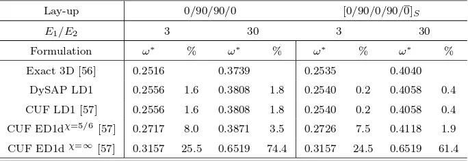
DySAP LD1 0.2556 1.6 0.3808 1.8 0.2540 0.2 0.4058 0.4 CUF LD1 [57] 0.2556 1.6 0.3808 1.8 0.2540 0.2 0.4058 0.4 CUF ED1dχ=5/6 [57] 0.2717 8.0 0.3871 3.5 0.2726 7.5 0.4118 1.9
CUF ED1dχ=∞
[57] 0.3157 25.5 0.6519 74.4 0.3157 24.5 0.6519 61.4
instance, for LD1-4, 3 DOF times 9 interfaces, times 3 nodes (2 elements) gives 81 DOF.
[image:46.612.123.486.332.436.2]It can observed that a lower number of fictitious interfaces are needed to obtain results close to the 3D exact solution for thin plies. This confirm that the important parameter when deciding how to model a composite plate is the thickness ratio of the single plies rather than the thickness ratio of the whole plate. Thicker plies and higher stiffness ration require more interfaces, i.e. higher order theories.
Table 3: Fundamental dimensionless bending frequencies ω∗ = ωhpρ/E2 and
percent-age error for a square SSSS plate with 2 different skew-symmetric staking sequences and
stiffness ratio. Convergence of the LD theory to the 3D exact solution by increasing the
number of interfaces.
Lay-up 0/90 [0/90]5
E1/E2 3 30 3 30
Formulation DOF ω∗ % ω∗ % DOF ω∗ % ω∗ %
Table 4: Fundamental dimensionless bending frequenciesω∗=ωhpρ/E
2and percentage
error for a square SSSS plate with 2 different symmetric staking sequences and stiffness
ratio. Convergence of the LD theory to the 3D exact solution by increasing the number
of interfaces.
Lay-up 0/90/90/0 [0/90/0/90/0]S
E1/E2 3 30 3 30
Formulation DOF ω∗
% ω∗
% DOF ω∗
% ω∗
% Exact 3D [56] 0.2516 0.3739 0.2535 0.4040 DySAP LD1-1 45 0.2556 1.6 0.3808 1.8 90 0.2540 0.2 0.4058 0.4 DySAP LD1-2 81 0.2522 0.2 0.3758 0.5 171 0.2536 0.0 0.4045 0.1 DySAP LD1-4 153 0.2517 0.1 0.3744 0.1 333 0.2535 0.0 0.4041 0.0
it is still an approximate method and requires a rather large number of DOF. DySAP LD1 on the other hand, with only 45 DOF, gives a closed form solu-tion, thus no loss of accuracy at higher frequencies. Furthermore, the DySAP LD1-8 model with 8 fictitious interfaces for each ply, i.e. a total of 153 DOF, show the same accuracy of the 3D FEM model with a fine mesh which has 4 order of magnitude more DOF (see Table (5)). It should also be observed that the 2D FE model show a relatively good accuracy for such a thick plate. This is surprising because the theory used in the 2D FE model should be an equivalent single layer (ESL) first order shear deformation theory (FSDT), equivalent to the one called CUF ED1d χ=5/6 in Table (1), which gives an error of 4.7% when compared with the results using 3D theory. The use of FSDT for composites raises some concerns about the shear correction factor
χ to be used. By changing that shear correction factor, the results can be changed rather significantly. For this plate material and stacking sequence it seems that the 2D results give a small error, but for other laminates, the error could be much higher [18–20, 57]. Layer wise theory (as well as high order ESL) do not need any shear correction factor and thus can be consid-ered much more reliable.
In Table (6), the same comparison is made for the first 10 natural frequen-cies. No 3D exact solution is available for higher frequencies thus the 3D fine mesh FE results are used for comparative purposes. It can be observed that DySAP LD1-8 shows a maximum error of 0.1 for all the frequencies with 153 DOF while, 2D FE result error increases for higher frequencies with a maximum error of 5% with 15606 DOF.
![Figure 1: Example of real stress and displacement fields for multilayered structures [5]](https://thumb-us.123doks.com/thumbv2/123dok_us/1502050.102924/5.612.160.451.348.434/figure-example-real-stress-displacement-elds-multilayered-structures.webp)