Structural optimisation of vertical-axis wind turbine composite
blades based on finite element analysis and genetic algorithm
Lin Wanga*, Athanasios Koliosa, Takafumi Nishinoa Pierre-Luc Delafina ,Theodore Birdb
a Centre for Offshore Renewable Energy Engineering, School of Energy, Environment and Agrifood, Cranfield University, Cranfield, MK43 0AL, UK
b
Aerogenerator Project Limited, Ballingdon Mill, Sudbury, CO10 7EZ, UK
Abstract
A wind turbine blade generally has complex structures including several layers of composite materials with
shear webs, making its structure design very challenging. In this paper, a structural optimisation model for
wind turbine composite blades has been developed based on a parametric FEA (finite element analysis)
model and a GA (genetic algorithm) model. The optimisation model minimises the mass of composite
blades with multi-criteria constraints. The number of unidirectional plies, the locations of the spar cap and
the thicknesses of shear webs are taken as design variables. The optimisation model takes account of five
constraints, i.e. stress constraint, deformation constraint, vibration constraint, buckling constraint, and
manufacturing manoeuvrability and continuity of laminate layups constraint. The model has been applied
to the blade structural optimisation of ELECTRA 30kW wind turbine, which is a novel VAWT
(vertical-axis wind turbine) combining sails and V-shape arm. The mass of the optimised blade is 228kg, which is
17.4% lower than the initial design, indicating the blade mass can be significantly reduced by using the
present optimisation model. It is demonstrated that the structural optimisation model presented in this
paper is capable of effectively and accurately determining the optimal structural layups of composite
blades.
Keywords: Vertical-axis wind turbine; Composite blade; Structural optimisation; Finite element analysis;
Genetic algorithm
Acronyms
APL Aerogenerator Power Limited
CBCSA Composite Blade Cross-Section Analysis
CLT Classical Lamination Theory
COE Cost of Energy
*
CTM4E Cranfield Turbine Model version 4E
DECC Department of Energy & Climate Change
EBSFT Extended Bredt-Batho Shear Flow Theory
ETI Energy Technologies Institute
FEA Finite Element Analysis
GA Genetic Algorithm
GL Germanischer Lloyd
HAWT Horizontal-Axis Wind Turbine
NAM_WTB Nonlinear Aeroelastic Model for Wind Turbine Blades
NOVA Novel Offshore Vertical Axis
PSO Particle Swarm Optimisation
SA Simulated Annealing
VAWT Vertical-Axis Wind Turbine
WindPACT Wind Partnership for Advanced Component Technologies
1D One-Dimensional
3D Three-Dimensional
Nomenclature
max
d Maximum blade deformation
allow
d Allowable deformation
x
E Longitudinal Young’s modulus
y
E Lateral Young’s modulus
blade
f First natural frequency of the blade
rotor
f Frequency of the rotor rotation
s
f Material safety factor
obj
F Objective function
xy
G Shear modulus
m
L Load multiplier
allow m
L _ Allowable load multiplier
B
m Mass of the blade
Ini
N Number of initial samples
MaxEval
N Maximum number of evaluations
MaxIter
N Maximum number of iterations
PerIter
ply
t Ply thickness
n
x x
x1, 2,, Design variables
L
x Lower bound of design variables
U
x Upper bound of design variables
X Row matrix that contains all design variables
xy
υ
Poisson’s ratioρ Material density
allow C,
σ
Allowable longitudinal compressive stressmax ,
C
σ
Maximum longitudinal compressive stressulti C,
σ
Ultimate longitudinal compressive stressallow T,
σ
Allowable longitudinal tensile stressmax ,
T
σ
Maximum longitudinal tensile stressulti T,
σ
Ultimate longitudinal tensile stressallow
∆ Allowable tolerance
1. Introduction
Deployment of offshore wind farms during the past decade has highlighted some difficulties associated
with conventional wind turbines. Conventional HAWTs (horizontal-axis wind turbines) place their main
components (such as the rotor and drive-train) at the top of very tall towers, making both installation and
maintenance difficult and limiting their size. VAWTs (vertical-axis wind turbines) can overcome the above
disadvantages by locating their main components at the base of the wind turbine, offering easy access for
both installation and maintenance. Additionally, VAWTs are insensitive to wind direction and therefore
there is no need for sophisticated yawing system, which significantly reduces the cost of the turbine.
Therefore, there has been a resurgence of interest in the development of VAWTs for offshore applications
[1-3].
The conventional VAWTs based on the Darrieus concept [4] encounter a large aerodynamic overturning
moment, which results in very heavy drive-train components. In order to minimise the aerodynamic
overturning moment, Sharpe [5] proposed a novel V-shape VAWT rotor, which combines a V-arm with
several sails positioned along the span. Fig. 1 presents a photograph of a 5kW prototype device developed
Figure 1. 5kW prototype device developed by Wind Power Ltd [6]
In 2009, ETI (Energy Technologies Institute) commissioned NOVA (Novel Offshore Vertical Axis) project
[7], which is a £2.8M feasibility study project to develop the concept design of a novel 10MW offshore
VAWT based on the novel V-shape rotor. Through case studies, it is demonstrated that using two
high-aspect-ratio (i.e. large span-to-chord ratio) sails is more aerodynamically efficient than multiple
low-aspect-ratio sails. This is due to the fact that the two-sail design experiences lower junction flows, which
result in lower interference drags. Therefore a new V-shape with two-sail concept design is proposed in the
NOVA project, as illustrated in Fig. 2.
[image:4.612.69.495.361.691.2]Based on the V-shape and two-sail concept, the ELECTRA 30kW vertical-axis wind turbine is currently
being developed in the 30kW Aerogenerator project, which is an on-going project (commenced in January
2015) and is funded by both DECC (Department of Energy & Climate Change) and APL (Aerogenerator
Power Limited). The ELECTRA 30kW turbine will be built and tested, and it will also be used to
demonstrate and generate information to scale up for offshore application.
Blades are key components of a wind turbine. The aerodynamic shape of a wind turbine blade is generally
optimised in order to achieve better power performance [8-10]. In terms of the structure, wind turbine
blades are generally made of composite materials due to their high strength-to-weight ratio and good
fatigue performance. In order to meet design requirements, wind turbine blades commonly have complex
structural layout, comprising one or more shear webs and a number of composite plies placed at different
ply angles [11, 12]. The structural performance of a composite blade can be tailored by changing stacking
sequence, fibre orientation, stacking location and size of the materials. Due to the inherent complexity of
composite materials and the complicated blade structural layout, optimisation of a composite blade is very
challenging and requires a specialised structural optimisation model.
In general, a structural optimisation model of wind turbine composite blades consists of two components,
i.e. 1) a blade structural model, which determines the structural performance of the blade, such as blade
mass and stress distributions; and 2) an optimisation algorithm, which handles the design variables and
searches for the optimal solutions.
Structural models used for wind turbine blades can be roughly categorised into two groups, i.e. 1D
(one-dimensional) beam model and 3D (three-(one-dimensional) FEA (finite element analysis) model. Due to its
efficiency and reasonable accuracy, beam model has been widely used in aeroelasticity analysis and
structural dynamics analysis of wind turbine blades. Based on a nonlinear beam model, Wang et al. [13]
developed a nonlinear aeroelastic model called NAM_WTB (Nonlinear Aeroelastic Model for Wind
Turbine Blades), which takes account of geometric nonlinearities and large blade deformations. The main
input data of the beam model are the sectional properties, such as mass per unit length and
cross-sectional stiffness, which can be calculated by using specialised cross-cross-sectional analysis models. An
example of such cross-sectional analysis models is CBCSA (Composite Blade Cross-Sectional Analysis)
[14], which is developed by Wang et al. through combining CLT (Classical Lamination Theory) [15] and
EBSFT (Extended Bredt-Batho Shear Flow Theory) [16]. Although it is efficient, the beam model is
incapable of offering some important information for the blade design, such as detailed stress distributions
within each layer of the blade structure. In order to obtain such detailed information, it is necessary to
construct the blade structure model using 3D FEA. In 3D FEA, wind turbine composite blades are
generally constructed using 3D composite shell elements, which are capable of describing composite layer
provides more accurate results and is able to predict detailed stress distributions within the blade structure.
For this reason, the 3D FEA model is chosen in this study to model the composite blade structure.
Optimisation algorithms used for wind turbine blades can be roughly categorised into three groups [17],
i.e. exact algorithms, heuristic algorithms and metaheuristic algorithms. Exact algorithms evaluate every
possible combination of design variables to find the best solution. It is a very accurate approach because all
possible combinations are evaluated. However, it becomes inefficient and even infeasible in cases of a
large number of design variables, requiring huge computational costs to evaluate all possible combinations.
Heuristic algorithms (also known as approximate algorithms) find near-optimal solutions based on
semi-empirical rules. Heuristic algorithms are more efficient than exact algorithms, but they are
problem-dependent and their accuracy depends on the accuracy of semi-empirical rules, limiting their applications
to some extent. Metaheuristic algorithms (also known as hyper-heuristics), which are more complex and
intelligent heuristics, are high-level problem-independent algorithms to find near-optimal solutions.
Metaheuristic algorithms are more efficient than common heuristic and are generally based on optimisation
processes observed in the nature, such as SA (simulated annealing), PSO (particle swarm optimisation) and
GA (genetic algorithm). Among these metaheuristic algorithms, the GA, which finds solutions to
optimisation problems using techniques inspired by genetics and natural evolution, has the ability to handle
a large number of design variables and to avoid being trapped in local optimal solution, making it the most
widely used metheuristic algorithm for the optimisation of wind turbine blades [18, 19]. For this reason,
the GA is chosen in this study to handle the design variables and to search for the optimal solutions.
To the best of the authors’ knowledge, the combination of FEA and GA for structural optimisation of
vertical-axis wind turbine blades has not been reported in the literature. This paper attempts to combine
FEA and GA to develop a structural optimisation model of wind turbine composite blades. A parametric
FEA model is developed, and then it is coupled with GA to develop a structural optimisation model. The
structural optimisation model is applied to the ELECTRA 30kW wind turbine blade, which is a novel
VAWT blade, to optimise the structural layout of the blade.
This paper is structured as follows. Section 2 illustrates the ELECTRA 30kW wind turbine blade. Section 3
presents the parametric FEA model of wind turbine composite blades. Section 4 presents the GA model.
Section 5 presents the optimisation model by combining the parametric FEA model and the GA model.
Results and discussions are provided in Section 6, followed by conclusions in Section 7.
2. ELECTRA 30kW Wind Turbine Blade
The wind turbine model used in the present study is the ELECTRA 30kW wind turbine, which is a novel
2-bladed VAWT combining V-shape and sails. The two blades of the turbine are designed to be identical, and
optimised by the 30kW Aerogenerator project team. In this study, a preliminary aerodynamic design of the
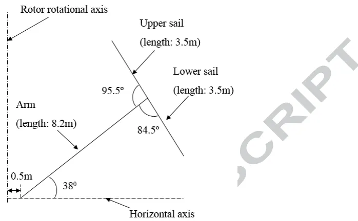
ELECTRA 30kW wind turbine blade is used, and its schematic is presented in Fig. 3.
Figure 3. Schematic of preliminary aerodynamic design of ELECTRA 30kW wind turbine blade
As can be seen from Fig. 3, the blade consists of three parts, i.e. arm, upper sail and lower sail. The length
of the arm is 8.2m, and the angle between the arm and the horizontal axis is 38º. The length of the upper
sail is 3.5m, and the angle between the upper sail and the arm is 95.5º. The length of the lower sail is 3.5m,
and the angle between the lower sail and the arm is 84.5º. The arm root offsets 0.5m from the rotor
rotational axis.
The preliminary aerodynamic design of the ELECTRA 30kW blade comprises two different airfoil shapes,
[image:7.612.190.539.98.314.2]i.e. NACA0040 and NACA0018, as shown in Table 1.
Table 1. Preliminary aerodynamic design of ELECTRA 30kW blade
Chord (m) Profile
Arm 0.6 NACA0040
Upper sail 0.8 NACA0018
Lower sail 0.8 NACA0018
3. Parametric FEA model
3.1. Model description
A parametric FEA model of wind turbine composite blades is established using ANSYS software [20]. It is
to create various blade models. The parametric FEA model can be applied to the FEA modelling of both
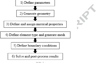
[image:8.612.157.541.118.372.2]horizontal-axis and vertical-axis wind turbine composite blades, and its flowchart is presented in Fig. 4.
Figure 4. Flowchart of the parametric FEA model.
Each step of the flowchart in Fig. 4 is detailed below.
1) Define parameters
In the first step, parameters involved in the FEA modelling, such as structure thickness and geometry data,
are defined.
2) Generate geometry
The blade geometry is generated based on the bottom-up approach, which generates low dimensional
entities (such as points) and build on top of them higher dimensional entities (such as lines and areas).
3) Define and assign material properties
In this step, material properties are defined and then assigned to the blade structure.
4) Define element type and generate mesh
In term of element type, the shell element shell281, which has eight nodes with six degrees of freedom at
each node, is used. The Shell281 element is well-suited for linear, large rotation, and/or large strain
nonlinear applications. It is also suitable for layered applications for modelling composite shells or
Additionally, a regular quadrilateral mesh generation method is utilised to create high quality elements.
5) Define boundary conditions
In this step, boundary conditions is applied. The types of boundary conditions depend on the types of
analysis. For example, for modal analysis, a fixed boundary condition is applied at the blade root.
6) Solve and post-process results
Having defined parameters, geometry, material, mesh, element properties and boundary conditions,
different types of analysis, such as static analysis, modal analysis and time-dependent analysis, can be
performed. The analysis results, such as deformations and stress distributions, are then plot using
post-processing functions of ANSYS software.
3.2. Validation of the parametric FEA model
A case study is performed in order to validate the parametric FEA model. The WindPACT 1.5MW wind
turbine [22-24], which is a representative of large-scale HAWTs, is chosen as an example. The reasons of
choosing a HAWT blade in the validation study are 1) HAWT blades have similar structures with VAWT
blades (for instance, both of them use airfoil cross sections made of composite materials); and 2) no data of
VAWT blades are publicly available for validation case studies.
WindPACT 1.5MW wind turbine is a reference wind turbine designed by NREL (National Renewable
Energy Laboratory) for the WindPACT (Wind Partnership for Advanced Component Technologies)
project between years 2000 and 2002. In the WindPACT project, the effects of the main wind turbine
components (such as blades and generator) on the cost of energy (COE) have been investigated. The
ultimate goal of the WindPACT project is to identify technology improvements to reduce the COE of wind
turbines in low-wind-speed sites. Details of the WindPACT project can be found in Ref. [25]. WindPACT
1.5MW wind turbine is a three-bladed HAWT, and its main parameters are summarised in Table 2. The
material properties and detailed structural layups of the WindPACT wind turbine blade can be found in
Ref. [24].
Table 2. Main parameters of the WindPACT 1.5MW wind turbine
Parameters Values
Rated power (MW) 1.5
Number of blades 3
Rotor radius (m) 35
The parametric FEA model presented in Section 3.1 is applied to the FEA modelling of the WindPACT
quality elements. The created mesh is depicted in Fig. 5, and a close view of the blade tip is presented in
[image:10.612.145.539.108.495.2]Fig. 6.
Figure 5. Mesh of WindPACT 1.5MW wind turbine blade
Figure 6. Close view of blade tip
The FEA model is used to perform modal analysis of the WindPACT 1.5MW wind turbine blade. In this
case study, the blade is non-rotating and free-vibration (no loads on the blade). A fixed boundary condition
is applied to the blade root. The results of the proposed FEA model are compared against the FEA results
Figure 7. Mode frequencies of WindPACT 1.5MW wind turbine blade
Table 3. Mode frequencies of WindPACT 1.5MW wind turbine blade
Mode frequencies Reference [24] Present %Diff
1st flapwise (Hz) 1.0783 1.0508 2.55
1st edgewise (Hz) 1.7001 1.7003 0.01
2nd flapwise (Hz) 2.9804 2.9329 1.59
2nd edgewise (Hz) 5.0382 4.9672 1.41
3rd flapwise (Hz) 6.3093 6.3978 1.40
4th flapwise (Hz) 10.305 10.034 2.63
As can be seen from Fig. 7 and Table 3, the flapwise and edgewise blade mode frequencies calculated
from the present FEA model show good agreement with the FEA results reported in Ref. [24], with the
maximum percentage difference (2.63%) occurring for the 4th edgewise mode. This confirms the validity of the present parametric FEA model.
3.3 Application of the parametric FEA model to the ELECTRA 30kW wind turbine
blade
The parametric FEA model is applied to the FEA modelling of the ELECTRA 30kW wind turbine blade.
The geometry, material properties, layout of the airfoil cross section, mesh, boundary conditions used in
the FEA modelling are presented below.
0 1 2 3 4
0 5 10 15 20 25
Mode
F
re
q
u
e
n
c
y
[
H
z
]
[image:11.612.131.481.363.491.2]3.3.1. Geometry
Based on the aerodynamic shape presented in Section 2, the 3D geometry of the ELECTRA 30kW wind
turbine blade is created, as depicted in Fig. 8. The circular arm root and arm tip are connected to the hub
and rectangular sail root using T-bolts, respectively. In this case study, for the sake of simplicity, the T-bolts
[image:12.612.232.538.172.329.2]and associated holes are not considered in the FEA modelling.
Figure 8. Geometry of the ELECTRA 30kW wind turbine blade
3.3.2. Material properties
The blade structure is designed to be made of five types of materials, i.e. gelcoat, random mat, DBM1708
(double-bias E-glass fibre), C260 (unidreictional E-glass fibre) and End-grain Balsa. The mechanical
properties of these materials are presented in Table 4. It should be noted that the materials for this study are
obtained from Refs. [26, 27] rather than manufacturing datasheets, as the real fabrication data are
[image:12.612.73.506.506.633.2]proprietary material and very challenging to obtain.
Table 4. Mechanical properties of materials [26, 27]
Material name Ex (GPa) Ey (GPa) Gxy (GPa) vxy ρ (kg/m3) tply (mm)
Gelcoat 3.44 3.44 1.38 0.3 1235 0.38
Random mat 7.58 7.58 4.00 0.30 1678 0.38
DBM1708 9.58 9.58 6.89 0.39 1814 0.89
C260 42.32 9.72 6.48 0.3 1737 0.6
End-grain balsa 0.12 0.12 0.02 0.3 230 -
3.3.3. Layout of the airfoil cross section
The airfoil cross section of the composite blade is presented in Fig. 9. As can be seen from Fig. 9, the blade
cross section is a three-cell section with two shear webs. The outermost skin of the cross section consists of
three layers, i.e. a gelcoat layer, a nexus layer and a double-bias-material composite laminate. The gelcoat
outer layer offers a smooth surface. Even though it is not a structural material, it can considerably
contribute to the blade mass. The nexus is a soft-material mat, protecting the rough surface of the
underlying double-bias laminate and providing an absorbent surface for the gelcoat. Double-bias layers are
mainly to provide shear strength and to avoid splaying of the unidirectional material. At both leading- and
trailing-edge panels, the double-bias laminate splits into two layers to accommodate a core material (e.g.
balsa), which augments the buckling strength of the blade.
A composite box-spar is enclosed in the midsection of the blade and is connected to the skin double-bias
layers at its lower and upper surfaces. The spar splits the cross section into three cells, with the
box-spar forming the mid-cell. The box-spar cap is mainly made of unidirectional composite laminates, which
provide most of the bending strength due to their good axial load-bearing capabilities. The two vertical
[image:13.612.75.440.354.623.2]sides of the box-spar serve as shear webs, consisting of double-bias composite laminate and core material.
Figure 9. Layout of airfoil cross section
3.3.4. Mesh
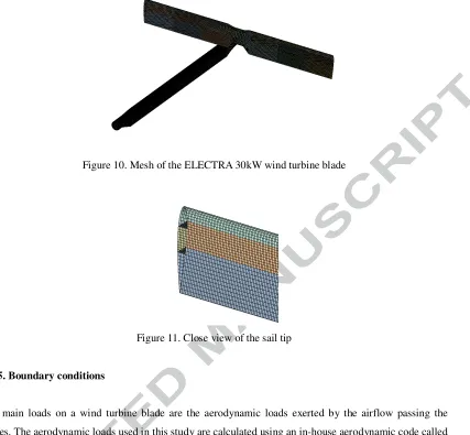
The mesh of the blade is presented in Fig. 10, and a close view of the sail tip is presented in Fig. 11. The
Figure 10. Mesh of the ELECTRA 30kW wind turbine blade
Figure 11. Close view of the sail tip
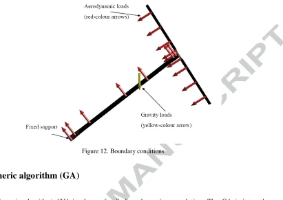
3.3.5. Boundary conditions
The main loads on a wind turbine blade are the aerodynamic loads exerted by the airflow passing the
blades. The aerodynamic loads used in this study are calculated using an in-house aerodynamic code called
CTM4E (Cranfield Turbine Model version 4E), which is developed by Shires [28] in the NOVA project.
The CTM4E code is based on Paraschivoiu’s DMST (Double-Multiple Streamtube) model [29], which
performs separate calculations of the induced velocity over upwind and downwind half-cycles of the rotor.
CTM4E code takes account of three-dimensional considerations for tip losses, tower losses and junction
drag. The CTM4E code has been validated by extensive benchmark tests [28], showing reasonable
agreement with experimental data.
The aerodynamic loads are calculated by CTM4E code under a 50-year extreme wind condition (wind
speed is 52.5m/s) with a parked rotor (i.e. rotor rotational speed is 0rpm). The overall aerodynamic
overturning moment on the blade root is 44.9kNm, taking account of a load safety factor of 1.35 according
to design standard IEC61400-2 [30]. The calculated aerodynamic loads are applied to the pressure-side of
the blade surface as distributed loads.
The boundary conditions used in the FEA modelling are presented in Fig. 12.
Figure 12. Boundary conditions
4. Generic algorithm (GA)
A GA (genetic algorithm) [31] is chosen for finding the optimum solution. The GA imitates the
fundamental principles of genetics and natural selection to constitute its optimisation procedures. In the
GA, a population of individuals (i.e. candidate solutions) to an optimisation problem is evolved gradually
toward better solutions. The evolution usually starts with an initial population, of which individuals are
created randomly. It is an iterative process, and the population in each iteration is called a generation. In
each generation, the fitness of each individual in the population is evaluated, and the fitness is usually the
value of the objective function of the optimisation problem. The individuals with high fitness values are
stochastically chosen from the present population. The genome of each individual is modified to form a
new generation through two ways, i.e. 1) mutation, which alters one or more gene values in a chromosome
from its initial state to form entirely new gene values being added to the gene pool; and 2) crossover,
which combines two chromosomes to produce a new chromosome. The new generation of individuals is
then used in the next iteration of the evolution. The evolution generally terminates when either the
population has reached a satisfactory fitness level, or a maximum number of generations has been
produced. The mutation and crossover used in the GA are briefly summarised below.
• Mutation
Mutation operator is analogous to biological mutation, and it alters one or more gene values in a
chromosome from their initial state. Mutation can contribute to entirely new gene values being added to
the gene pool, possibly resulting in a better solution. Mutation plays a significant role in the genetic search,
optima. A specified mutation probability is generally used to control the occurrence of mutation during
evolution. This probability should not be too high. Otherwise, the genetic search will become a basic
random search.
• Crossover
Crossover plays an important role in generating a new generation. Crossover mates (combines) two
chromosomes (parents) to generate a new chromosome (offspring). The basic idea behind crossover is that
the new chromosome might be better than both of the parents in cases that it takes the best characteristics
from each parent.
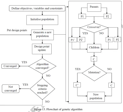
GA searches optimal solutions through an iterative procedure, which is presented below.
1) Define objectives, variables and constraints
The first step of GA is to define optimisation objectives, design variables and constraints.
2) Initialise population
In this step, GA randomly generates the initial population (samples). Large initial population set increases
the chance to find the input design variable space that contains the best solutions.
3) Generate a new population
In this step, GA generates a new population through mutation and crossover.
4) Design point update
In this step, the design points in the new population are updated.
5) Convergence validation
The optimisation converges when the convergence criteria have been reached. If the optimisation is not
converged, the evolution process continues to the next step.
6) Stopping criteria validation
If the optimisation has not yet converged, it is then further validated for fulfilment of stopping criterion,
i.e. the maximum number of iterations criterion. If the iteration number exceeds the maximum number of
iterations, the optimisation process is stopped without having reached convergence. Otherwise, the
optimisation process returns to Step 3 to generate a new population.
The above Steps 3 to 6 are repeated in sequence until the optimisation has converged or the stopping
Figure 13. Flowchart of genetic algorithm
5.
Structural optimisation model of composite blades
5.1. Objective function
In order to reduce the material cost of the wind turbine blade, the blade structure is required to be designed
as light as possible. Moreover, the lighter blade mass can also be beneficial to reduce both centrifugal and
gravity loads on the blade. Therefore, the minimum blade mass is taken as the objective function,
expressed as:
(
B)
obj m
F = min (1)
where obj
5.2. Design variables
Figure 14 presents the schematic of the blade structure. As can be seen from Fig. 14, the blade structure is
divided into 16 regions, including 7 regions on the arm and 9 regions on the sail. ArmRoot and
ArmRootTran are arm-root region and arm-root transition region, respectively. ArmAF1, ArmAF2 and
ArmAF3 are arm airfoil regions. ArmTipTran and ArmTip are arm-tip transition region and arm-tip region,
respectively. SailRoot, SailUpTran and SailDownTran are sail-root region, upper-sail transition region and
lower-sail transition region, respectively. SailUpAF1, SailUpAF2 and SailUpAF3 are upper-sail airfoil
regions. SailDownAF1, SailDownAF2 and SailDownAF3 are lower-sail airfoil regions. The materials used
in the structural design (i.e. gelcoat, random mat, double-bias plies, unidirectional plies and balsa) are
[image:18.612.80.514.175.708.2]presented in Section 3.3.2.
Figure 14. Schematic of the blade structure
Compared to unidirectional plies, the double-bias plies usually offers a much lower stiffness along the
blade. The main role of the double-bias plies is to prevent splaying of the unidirectional plies and to
provide shear strength. The shear-strength criteria might not yield any requirement for double-bias plies, as
wind turbine blades are generally subjected to low torsion loads. Therefore, an empirical value of 2 is
chosen as the number of double-bias plies. A single layer is used for the non-structure materials, i.e.
gelcoat and random mat. Table 5 presents the number of layers of gelcoat, random mat and double-bias
plies used in the blade structural design. The thickness of a single layer in Table 5 is the ply thickness tply
Table 5. Number of layers of double-bias plies, gelcoat and random mat
Item Number of layers Thickness of a single layer [mm]
Gelcoat 1 0.38
Random mat 1 0.38
Bouble-bias E-glass 2 0.6
The unidirectional plies carry most of the bending loads, and they generally contribute most of the overall
weight of the blade. In addition, the location of the spar cap and the thickness of the shear webs can also
significantly affect the weight of the blade. Therefore, the number of unidirectional plies, the location of
the spar cap and the thickness of shear webs are taken as design variables. The thickness of the core
material (i.e. balsa) at both airfoil leading- and trailing-edge panels is designed be identical to the thickness
of the unidirectional plies in the spar cap, in order to have a smooth transition between the panel and the
spar cap to avoid local stress concentration.
Thus, twenty-three design variables in total are defined, which can be expressed in the following form:
[
1 2]
=
23
=
x
x
x
n
X
nT
,
(2)where x1 is the number of unidirectional plies of the arm-root region; x2 is the number of unidirectional
plies of the arm-root transition region; x3, x4 and x5 are the number of unidirectional plies in the spar
cap of the arm airfoil regions; x6 is the number of unidirectional plies of the arm-tip transition region; x7
is the number of unidirectional plies of the arm-tip region;
x
8 is the number of unidirectional plies of thesail-root region;
x
9 is the number of unidirectional plies of the upper-sail transition region;x
10, x11and12
x
are the number of unidirectional plies of the upper-sail airfoil regions;x
13 is the number ofunidirectional plies of the lower-sail transition region;
x
14 , x15andx
16 are the number of unidirectionalplies of the lower-sail airfoil regions;
x
17,x
18 andx
19 are the thickness of shear webs of the arm, uppersail and lower sail, respectively;
x
20 andx
21 are the normalized chordwise locations of spar cap of thearm;
x
22 andx
23 are the normalized chordwise locations of spar cap of both upper sail and lower sail.5.3. Constraints
The structural optimisation of wind turbine composite blades requires multiple criteria to be taken into
account. In many cases, these criteria are mutually incomparable and sometimes even contradictory.
In this paper, five constraint conditions are taken into account, i.e. stress constraint, deformation constraint,
vibration constraint, buckling constraint, and manufacturing maneuverability and continuity of laminate
• Stress constraint
The tensile and compressive stresses generated by the loads cannot exceed associated allowable stresses.
This can be expressed in the following inequality forms:
allow T T,max
σ
,σ
≤ (3)allow C C,max
σ
,σ
≤ (4)where
σ
T,max is the maximum longitudinal tensile stress of the blade,σ
T,allow is the allowablelongitudinal tensile stress of the material,
σ
C,max is the maximum longitudinal compressive stress of theblade,
σ
C,allow is the allowable longitudinal compressive stress of the material.allow T,
σ
andσ
C,allow in Eqs. (3) and (4) are respectively given by the following equations:s ulti T allow
T,
σ
, / fσ
= (5)s ulti C allow
C,
σ
, / fσ
= (6)where
σ
T,ulti is the ultimate longitudinal tensile stress,σ
C,ulti is the ultimate longitudinal compressivestress,
s
f is the material safety factor.
According to GL (Germanischer Lloyd) design standard [32] and Refs. [33, 34], the material safety factor
s
f for wind turbine composite blades is 2.204. According to Ref. [27], the ultimate stresses
σ
T,ulti andulti C,
σ
of the unidirectional E-glass fibre C260 are 709.9MPa and 343.2MPa , respectively. Thus, theallowable stresses
σ
T,allow andσ
C,allow are respectively 322.1MPa and 155.7MPa, taking account of amaterial safety factor of 2.204.
• Deformation constraint
In order to avoid the uncertainties introduced by large blade deformations, the maximum blade
deformation dmax should not exceed the allowable deformation
allow
d . This can be expressed in the
following inequality form:
allow d
dmax ≤ (7)
The allowable deformation
allow
d in this study is set to 0.7m, which is 20% of the length of upper sail.
This small allowable deformation avoids the uncertainties introduced by large deformations.
In order to avoid the occurrence of resonance, the natural frequency of the composite blade should be
separated from the harmonic vibration associated with rotor rotation. This can be expressed in the
following inequality form:
allow rotor
blade f
f − ≥∆ (8)
where fblade is the first natural frequency of the blade, frotor is the frequency of the rotor rotation, ∆allow
is the associated allowable tolerance.
The maximum rotor rotational speed of ELECTRA wind turbine is 50rpm, and the associated frequency
rotor
f
is 0.833Hz. ∆allow is assumed to be 10% off
rotor , and thus the following inequality form isobtained: Hz .92 0 ≥ blade f (9)
• Buckling constraint
Due to buckling, composite materials under axial compression are generally weaker than those under axis
tension. The load multiplier Lm, which is the ratio of the critical buckling load to the applied load on the blade, should be larger than the allowable load multiplier Lm_allow. This can be expressed in the following
inequality form:
allow m
m L
L ≥ _ (10)
In this study, an empirical value of 1.5 is chosen for the allowable load multiplier Lm_allow.
• Manufacturing maneuverability and the continuity of laminate layups
Considering the manufacturing maneuverability and the continuity of the laminate layup, the following
constraints are applied to the design variables:
23 2 1, ,,
= ≤
≤ x x i
x i Ui
L
i (11)
4 3 2 1 0
1≥ = , , ,
− j + arm
j x j
x arm arm (12) 11 10 9 8 0
1 ≥ = , , ,
− j + SailUp
j x j
x
SailUp
SailUp (13)
0
13 8−x ≥
x (14)
15 14 13 0
1≥ = , ,
− j + SailDown
j x j
x
SailDown
SailDown (15)
where xL is the lower bound of the design variables; xU is the upper bound of the design variables.
The lower and upper bounds of the design variables and the constraint conditions are presented in Table
Table 6. Lower and upper bounds of the design variables and the constraint conditions
Design variable Lower bound Upper bound Units
ArmRoot
x
1 1 80 -ArmRootTran
x
2 1 70 -ArmAf1
x
3 1 60 -ArmAf2
x
4 1 50 -ArmAf3
x
5 1 40 -ArmTipTran
x
6 1 50 -ArmTip
x
7 1 60 -SailRoot
x
8 1 60 -SailUpTran
x
9 1 50 -SailUpAf1
x
10 1 40 -SailUpAf2
x
11 1 30 -SailUpAf3
x
12 1 20 -SailDownTran
x
13 1 50 -SailDownAf1
x
14 1 40 -SailDownAf2
x
15 1 30 -SailDownAf3
x
16 1 20 -ArmWeb
x
17 5 15 mmSailUpWeb
x
18 5 15 mmSailDownWeb
x
19 5 15 mmArmSparLoc1
x
20 0.15 0.3 -ArmSparLoc2
x
21 0.35 0.5 -SailSparLoc1
x
22 0.15 0.3 -SailSparLoc2
x
23 0.35 0.5 -T
σ 322.1 MPa
C
σ 155.7 MPa
max
d 0.7 m
blade
f 0.92 Hz
m
5.4. Parameter settings of genetic algorithm
GA presented in Section 4 is chosen as the optimisation algorithm, and the main parameter settings of GA
[image:23.612.81.533.155.627.2]are presented in Table 7.
Table 7. Main parameter settings of GA
Parameter name Value
Type of initial sampling Constrained sampling
Number of initial samples
N
Ini 230Number of samples per iteration
N
PerIter 50Maximum allowable Pareto Percentage [%] 70
Convergence stability percentage [%] 2
Maximum number of iterations
N
MaxIter 30Mutation probability 0.01
Crossover probability 0.82
Each parameter in Table 7 is detailed below.
• Type of initial sampling
The initial sampling is generated using constrained sampling algorithm, which constrains the sampling
using variable relationships defined in Eqs. (11) to (15).
• Number of initial samples
In this study, the number of initial samples
N
Ini is 230, which is 10 times the number of design variables.• Number of samples per iteration
In this study, an empirical value of 50 is chosen as the number of samples per iteration
N
PerIter.• Maximum allowable Pareto percentage
This parameter is a convergence criterion. Pareto percentage is defined as the ratio of the number of
desired Pareto points to the number of samples per iteration. When this percentage reaches the maximum
• Convergence stability percentage
Convergence stability percentage, which represents the stability of the population based on its mean and
standard deviation, is a convergence criterion. When this percentage (2% in this study) is reached, the
optimisation is converged.
• Maximum number of iterations
The maximum number of iterations, which is the maximum possible number of iterations the algorithm
executes, is a stop criterion. If this number (30 in this study) is reached without the optimisation having
reached convergence, the iteration will stop. It also provides an idea of the absolute maximum number of
evaluations
N
MaxEval, which is given by the following equation:(
−
1
)
∗
+
=
Ini PerIter MaxIterMaxEval
N
N
N
N
(16)where
N
Ini is the number of initial sampling,N
PerIter is the number of samples per iteration,N
MaxIter isthe maximum number of iterations.
• Mutation probability
Mutation probability, which defines the probability of applying a mutation on a design configuration, must
be between 0 and 1. A larger value indicates a more random algorithm. For instance, if the value is 1, the
algorithm becomes a pure random search. In this study, a typical value of 0.01 [35] is used for the
probability of mutation.
• Crossover probability
Crossover probability, which defines the probability with which parent solutions are recombined to
produce the offspring solutions, must be between 0 and 1. A smaller value indicates a more stable
population and a faster (but less accurate) solution. For instance, if the value is 0, the parents are directly
copied to the new population. In this study, a typical value of 0.82 [36] is used for the probability of
crossover.
5.5. Flowchart of the optimisation model
Figure 15 presents the flowchart of the optimisation model, which combines the parametric FEA model
Figure 15. Flowchart of the optimisation model
[image:25.612.86.537.62.634.2]6. Results and discussions
Figure 16 presents the history of the objective function (mass of the blade) during the optimisation process.
As can be seen from Fig. 16, the mass of the blade oscillates in the first few iterative steps and then
gradually converges, reaching the best result with a mass of 228 kg at the 28th iteration. The optimal blade design leads to a mass reduction of 17.4% in comparison with the initial design (the initial blade mass at
Figure 16. History of blade mass
Figs. 17 to 21 present the history of the maximum total deformation, maximum tensile stress, maximum
compressive stress, first natural frequency of the blade and buckling load multiplier, respectively. The
associated allowable values (i.e. upper/lower bounds) are also presented in these figures. As can be seen
from Figs. 17 to 21, the maximum compressive stress is quite close to the allowable values, while other
constraint parameters have relatively large margins from the allowable values. This indicates the
compressive stress is the dominant parameter in the design in the present case. Choosing another
[image:26.612.74.459.454.695.2]composite material with higher compressive strength would further reduce the blade mass.
Figure 17. History of maximum total deformation
0 200 400 600 800 1000 1200 1400
220 240 260 280 300 320 340
Number of design samples
B la d e m a s s [ k g ]
History of blade mass
0 200 400 600 800 1000 1200 1400
0 0.1 0.2 0.3 0.4 0.5 0.6 0.7 0.8 0.9 1
Number of design samples
M a x im u m t o ta l d e fo rm a ti o n [ m ]
[image:27.612.68.542.84.595.2]
Figure 18. History of the maximum tensile stress
Figure 19. History of the maximum compressive stress
0 200 400 600 800 1000 1200 1400
100 150 200 250 300 350
Number of design samples
M a x im u m t e n s ile s tr e s s [ M P a
] History of maximum tensile stressUpper Bound
0 200 400 600 800 1000 1200 1400
90 100 110 120 130 140 150 160 170
Number of design samples
M a x im u m c o m p re s s iv e s tr e s s [ M P a ]
[image:28.612.154.537.84.323.2]
Figure 20. History of first natural frequency of the blade
Figure 21. History of buckling load multiplier
The optimised results of design variables, which have been rounded up, are presented in Table 8. As can be
seen from Table 8, all design variables meet the constraints defined in Eqs. (11) to (15).
0 200 400 600 800 1000 1200 1400
0.85 0.9 0.95 1 1.05 1.1 1.15 1.2 1.25
Number of design samples
B la d e f ir s t fr e q u e n c y [ H z ]
History of blade first frequency Lower Bound
0 200 400 600 800 1000 1200 1400
1.4 1.6 1.8 2 2.2 2.4 2.6 2.8 3 3.2 3.4
Number of design samples
B u c k lin g l o a d m u lt ip lie r
Table 8. Optimised results of design variables
Design variable Optimal value Unite
1
x
40-2
x
22-3
x
21-4
x
13-5
x
3-6
x
19-7
x
25-8
x
33-9
x
21-10
x
17-11
x
8-12
x
6-13
x
20-14
x
16 -15
x
10 -16
x
5 -17
x
8.8 mm18
x
8.5 mm19
x
7.5 mm20
x
0.203 -21
x
0.388 -22
x
0.229 -23
x
0.387 -The blade stress distributions, deformations, first modal frequency, and buckling analysis results for the
optimised blade are presented below.
• Stress distributions
Figure 22 presents the normal stress distributions within the blade structure. From Fig. 22 we can see that
than the allowable value of 322.1MPa; and 2) the absolute value of maximum negative normal stress (i.e.
[image:30.612.123.538.107.327.2]maximum compressive stress) is 151.28MPa, which is quite close to the allowable value of 155.7MPa.
Figure 22. Normal stress distributions of the blade structure
• Blade deformations
Figure 23 presents the total deformations of the blade. The un-deformed wireframe is also presented in this
figure to facilitate the illustration. As can be seen from Fig. 23, the maximum total deformation is about
0.593m, observed at the tip of the upper sail. This value is 15.3% lower than the allowable value of 0.7m,
[image:30.612.168.469.466.669.2]indicating the present blade design is quite stiff and is not likely to experience large deformations.
• Modal frequencies and shapes
The modal analysis is used to obtain the dynamic properties of the blade, such as modal frequencies and
modal shapes. In this case, the blade is non-rotating and free-vibration (no loads on the blade). Fig. 24
presents the frequency and modal shape of the first mode of the blade. As can be seen from Fig. 24, the
[image:31.612.113.535.130.415.2]mode frequency is about 1.0Hz, which is 8.7% higher than the allowable value of 0.92Hz.
Figure 24. Modal frequency and modal shape of first mode of the blade
• Buckling analysis results
Due to buckling, composite materials under axial compression are generally weaker than those under axis
tension. Fig. 25 presents the buckling analysis results of the blade. As can be seen from Fig. 25, the load
multiplier is about 2.15, which is 43.33% higher than the allowable value of 1.5. This indicates the present
Figure 25. Buckling load multiplier and buckling mode shape of the blade
7. Conclusions
In this work, a structural optimisation model for wind turbine composite blades has been developed by
combining 1) a parametric FEA (finite element analysis) model, which provides a high-fidelity solution of
the global behaviour of the blade; with 2) a GA (generic algorithm) model, which handles the design
variables and searches for the optimal solutions. The structural optimisation model minimises the mass of
the blade with multi-criteria constraint conditions. The number of unidirectional plies, the location of the
spar cap and the thickness of shear webs are taken as the design variables. The optimisation model takes
account of five constraint conditions, i.e. stress constraint, deformation constraint, vibration constraint,
buckling constraint, and manufacturing maneuverability and continuity of laminate layups constraint. The
model was applied to the blade structural optimisation of ELECTRA 30kW wind turbine, which is a novel
vertical-axis wind turbine combining sails and V-shape arm. The following conclusions can be drawn from
the present study:
• Good agreement (with maximum percentage difference of 2.63%) is achieved in comparison with the
modal analysis results of WindPACT 1.5MW wind turbine composite blade reported in the literature,
confirming the validity of the parametric FEA model developed in the present study.
• The structural optimisation model developed in this paper is capable of effectively and accurately
determining the optimal structural layups of composite blades, significantly improving the efficiency
of blade structural optimisation.
• The mass of the optimised blade is 228kg, which is 17.4% lower than the initial design, indicating the
• For the optimal blade, the maximum compressive stress is quite close to the allowable values, while
other constraint parameters (i.e. maximum total deformation, maximum tensile stress, first natural
frequency of the blade and buckling load multiplier) have relatively large margins from the allowable
values. This indicates the compressive stress is the dominant parameter in the presented design case.
Choosing another composite material with higher compressive strength would further reduce the blade
mass.
• The present model can be used for any practice of structural optimisation of wind turbine composite
blades, minimising the blade mass with multi-criterion constraint conditions.
Acknowledgements
Authors gratefully acknowledge the financial support of UK Government’s Department of Energy &
Climate Change and Aerogenerator Project Limited, who is the IP holder of the ELECTRA vertical axis
wind turbine configuration concept.
References
[1] A. Kolios, A. Chahardehi, and F. Brennan, "Experimental determination of the overturning moment and net lateral force generated by a novel vertical axis wind turbine: experiment design under load
uncertainty," Experimental Techniques, vol. 37, pp. 7-14, 2013.
[2] L. Wang, A. Kolios, P.-L. Delafin, T. Nishino, and T. Bird, "Fluid Structure Interaction Modelling of A Novel 10MW Vertical-Axis Wind Turbine Rotor Based on Computational Fluid Dynamics and Finite Element Analysis," presented at the EWEA 2015 Annual Event, Paris, France, 2015.
[3] M. Borg, M. Collu, and A. Kolios, "Offshore floating vertical axis wind turbines, dynamics modelling state of the art. Part II: Mooring line and structural dynamics," Renewable and Sustainable Energy Reviews, vol. 39, pp. 1226-1234, 2014.
[4] M. H. Worstell, "Aerodynamic performance of the DOE/Sandia 17-m-diameter vertical-axis wind turbine," Journal of Energy, vol. 5, pp. 39-42, 1981.
[5] D. J. Sharpe, "Vertical axis turbine apparatus," ed: Google Patents, 2011.
[6] J. Chatterton, D. Parsons, J. Nicholls, P. Longhurst, M. Bernon, A. Palmer, et al., "Carbon brainprint– An estimate of the intellectual contribution of research institutions to reducing greenhouse gas emissions," Process Safety and Environmental Protection, vol. 96, pp. 74-81, 2015.
[7] D. J. Parsons, J. C. Chatterton, F. P. Brennan, and A. J. Kolios, "Carbon Brainprint Case Study: novel offshore vertical axis wind turbines," Cranfield University, 2011.
[8] X. Liu, L. Wang, and X. Tang, "Optimized linearization of chord and twist angle profiles for fixed-pitch fixed-speed wind turbine blades," Renewable Energy, vol. 57, pp. 111-119, 2013.
[9] L. Wang, X. Tang, and X. Liu, "Blade design optimisation for fixed-pitch fixed-speed wind turbines,"
ISRN Renewable Energy, vol. 2012, 2012.
[10] L. Wang and X. Liu, "Optimized chord and twist angle distributions of wind turbine blade considering Reynolds number effects," in Wind Energy: Materials, Engineering and Policies (WEMEP), 2012. [11] G. S. Bir and P. G. Migliore, Preliminary structural design of composite blades for two-and three-blade
rotors: Citeseer, 2004.
[12] L. Wang, "Nonlinear aeroelastic modelling of large wind turbine composite blades," University of Central Lancashire, 2015.
[13] L. Wang, X. Liu, N. Renevier, M. Stables, and G. M. Hall, "Nonlinear aeroelastic modelling for wind turbine blades based on blade element momentum theory and geometrically exact beam theory,"
[14] L. Wang, X. Liu, L. Guo, N. Renevier, and M. Stables, "A mathematical model for calculating
cross-sectional properties of modern wind turbine composite blades," Renewable Energy, vol. 64, pp. 52-60, 2014.
[15] J. N. Reddy, Mechanics of laminated composite plates and shells: theory and analysis: CRC press, 2004.
[16] M. Shama, Torsion and shear stresses in ships: Springer Science & Business Media, 2010. [17] J. F. Herbert-Acero, O. Probst, P.-E. Réthoré, G. C. Larsen, and K. K. Castillo-Villar, "A Review of
Methodological Approaches for the Design and Optimization of Wind Farms," Energies, vol. 7, pp. 6930-7016, 2014.
[18] H. Xuan, Z. Weimin, L. Xiao, and L. Jieping, "Aerodynamic and aeroacoustic optimization of wind turbine blade by a genetic algorithm," in Proceedings of 46th AIAA Aerospace Sciences Meeting and Exhibit, 2008, pp. 2008-1331.
[19] K. Yassin, A. Diab, and Z. Ghoneim, "Aerodynamic Optimization of a Wind Turbine Blade Designed for Egypt's Saharan Environment Using a Genetic Algorithm," Renewable Energy and Sustainable Development, vol. 1, pp. 106-112, 2015.
[20] ANSYS, "Version 15.0; ANSYS," Inc.: Canonsburg, PA, USA November, 2013. [21] ANSYS, "ANSYS help documentation," Inc.: Canonsburg, PA, USA November, 2013.
[22] D. Malcolm and A. Hansen, "WindPACT turbine rotor design study," National Renewable Energy Laboratory, Golden, CO, vol. 5, 2002.
[23] D. A. Griffin, "WindPACT Turbine design scaling studies technical area 1œComposite blades for 80-to 120-meter rotor," National Renewable Energy Laboratory Technical report, 2001.
[24] B. Resor and T. Bushnell, "A 1.5 MW NuMAD Blade Model," Draft Report, Sandia National Laboratories, Albuquerque, NM, 2011.
[25] http://www.nrel.gov/wind/windpact.html; accessed 28-July-2014.
[26] D. Berry and T. Ashwill, "Design of 9-meter carbon-fiberglass prototype blades: CX-100 and TX-100,"
SAND2007-0201, Sandia National Laboratories, Albuquerque, NM, 2007.
[27] J. W. Lee, S. N. Gangadharan, and M. Mirmirani, "A Baseline Study and Calibration for Multidisciplinary Design Optimization of Hybrid Composite Wind Turbine Blade," in 52nd AIAA/ASME/ASCE/AHS/ASC Structures, Structural Dynamics and Materials Conference 19th AIAA/ASME/AHS Adaptive Structures Conference 13t, 2011, p. 1902.
[28] A. Shires, "Development and evaluation of an aerodynamic model for a novel vertical axis wind turbine concept," Energies, vol. 6, pp. 2501-2520, 2013.
[29] I. Paraschivoiu, "Double-multiple streamtube model for studying vertical-axis wind turbines," Journal of propulsion and power, vol. 4, pp. 370-377, 1988.
[30] I. Commission, "IEC 61400-2: Wind Turbines–Part 2: Design requirements for small wind turbines," ed: IEC, 2006.
[31] S. Sivanandam and S. Deepa, Introduction to genetic algorithms: Springer Science & Business Media, 2007.
[32] G. W. Guideline and G. Lloyd, "Guideline for the certification of Wind Turbines," Hamburg: Germanischer Lloyd Wind Energie Gmb H, 2010.
[33] C. Bak, F. Zahle, R. Bitsche, T. Kim, A. Yde, L. Henriksen, et al., "The DTU 10-MW reference wind turbine," Danish wind power research, 2013.
[34] D. T. Griffith and T. D. Ashwill, "The Sandia 100-meter all-glass baseline wind turbine blade: SNL100-00," Sandia National Laboratories, Albuquerque, Report No. SAND2011-3779, 2011.
[35] R. E. Perez, J. Chung, and K. Behdinan, "Aircraft conceptual design using genetic algorithms," AIAA Paper, vol. 4938, 2000.
![Figure 2. Concept design of NOVA 10MW wind turbine [7]](https://thumb-us.123doks.com/thumbv2/123dok_us/1566703.109257/4.612.220.539.65.308/figure-concept-design-of-nova-mw-wind-turbine.webp)


![Table 4. Mechanical properties of materials [26, 27]](https://thumb-us.123doks.com/thumbv2/123dok_us/1566703.109257/12.612.73.506.506.633/table-mechanical-properties-materials.webp)