Multichannel Spectral Factorization Algorithm
Using Polynomial Matrix Eigenvalue Decomposition
Zeliang Wang
∗, John G. McWhirter
∗and Stephan Weiss
† ∗School of Engineering, Cardiff University, Cardiff, Wales, UK†Department of Electronic & Electrical Engineering, University of Strathclyde, Glasgow, Scotland, UK
Email: [email protected], [email protected], [email protected]
Abstract—In this paper, we present a new multichannel spectral factorization algorithm which can be utilized to cal-culate the approximate spectral factor of any para-Hermitian polynomial matrix. The proposed algorithm is based on an iterative method for polynomial matrix eigenvalue decomposition (PEVD). By using the PEVD algorithm, the multichannel spectral factorization problem is simply broken down to a set of single channel problems which can be solved by means of existing one-dimensional spectral factorization algorithms. In effect, it transforms the multichannel spectral factorization problem into one which is much easier to solve.
I. INTRODUCTION
Spectral factorization arises in the analysis and design of linear systems, such as constructing a causal system which corresponds to a given spectral density function. The concept was initially introduced by Wiener to factorize the spectrum of a random sequence [1], and has been further extended to multivariate sequence scenarios [2]. Since then, Youla [3] established the fundamental results on rational spectral matrix factorization problems.
There exist numerous algorithms for calculating spectral factorization, such as a Newton-Raphson based method pro-posed by Wilson for the scalar case [4] and the polynomial matrix case [5], and the spectral factorization algorithm de-veloped by Janashiaet al.[6]. A paper written by Kuˇcera [7] illustrated some major parametric methods for calculating the spectral factorization, including Toeplitz matrix decomposition and Newton-Raphson iterations. Each method has its own advantages to cope with spectral factorization, but none of them is perfect. They are only suitable under certain circum-stances. Newton-Raphson’s method converges fast at the cost of high computational complexity, while the Toeplitz matrix decomposition converges more slowly with less computational cost. In addition, a paper written by Sayed [8] presented a survey of spectral factorization methods including the Bauer method, the Schur algorithm, the Levinson-Durbin algorithm, and techniques based on the Riccati equation, the Kalman filter and so on.
Most of these spectral factorization algorithms, with the exception of those due to Wilson and Janashia, do not extend to the multichannel situation. Wilson’s algorithm seems to provide a viable approach to the multichannel spectral fac-torization problem in terms of stability and reliability but is reputed to run into problems when the number of channels grows too big.
Spectral factorization has attracted lots of interest in dig-ital signal processing and communications in recent years. Applications have been found in areas, such as designing minimum phase FIR filters, quadrature-mirror filter banks [9], the optimum transmit and receive filter matrices for precoding and equalization of multiple-input multiple-output (MIMO) systems [10], and minimum phase FIR precoders for multicasting MIMO frequency selective channels [11].
The contribution of this paper is to study a novel method in computing the multichannel spectral factorization, and this method utilizes an iterative PEVD algorithm, known as the second order sequential best rotation (SBR2) algorithm [12], to break down the multichannel spectral factorization problem into independent single channel spectral factorization problems for which suitable algorithms already exist. In addition, the fundamental indeterminacy property of spectral factorization has been exploited in order to keep the resulting spectral factor order as low as possible.
For the rest of the paper, we start by formulating the multichannel spectral factorization problem in Sec. II. In Sec. III, an iterative PEVD algorithm, i.e. the SBR2 algo-rithm, is briefly introduced. Sec. IV describes the proposed multichannel spectral factorization method. Simulation results and conclusions are shown in Sec. V and Sec. VI respectively.
II. PROBLEMFORMULATION
In many signal processing applications involving multiple sensors, given a data vector x[n] ∈ CM
, the space-time co-variance matrix is represented byR[τ] =Ex[n]xH[n−τ] , in whichE{·}denotes the expectation, and the superscript H stands for Hermitian transpose. Thus the cross-spectral density (CSD) matrix R(z) is computed by applying z-transform to R[τ], s.t. R(z) = PτR[τ]z−
τ
. Note that the CSD matrix is a para-Hermitian polynomial matrix, which satisfies
e
R(z) =R(z). Here Re(z)is the paraconjugate of R(z), and it is defined as Re(z) = RH(1/z), i.e. applying Hermitian transpose to the polynomial coefficient matrices R[τ] and time-reversing all the elements in it.
According to Wiener’s spectral factorization theorem [2], [6], [13], if a para-Hermitian polynomial matrix R(z) is positive definite on the unit circle|z|= 1, and ifdet{R(ejθ)} satisfies the Paley-Wiener condition
Z π
−π
ln det{R(ejθ)}dθ <∞ ,
thenR(z)has a spectral factorization
R(z) =R+(z)R−(z) =R+(z)Re+(z) , (2)
whereR+(z)andR−(z)are respectively defined as anouter
and innerspectral factor [6], and R−(z) is paraconjugate of R+(z), i.e.R−(z) =Re+(z).
Note that an outer spectral factor R+(z) is not unique due to the fundamental indeterminacy in spectral factorization whereby ifR+(z)is a validouterspectral factor ofR(z)so also is R+(z)U(z) where U(z) represents any paraunitary polynomial matrix which preserves the essential properties associated with anouter spectral factor. This includes simple examples such asU(z) =zTI,U(z) =SwhereSis a simple unitary matrix, or the case in whichU(z)takes the form of a diagonal matrix with each entry given by a power ofzwhich need not be the same for all entries.
According to [6], [10], [14], the outer spectral factor R+(z) = Pτ≥0R+[τ]zτ in (2) is unique up to a constant unitary factor C, s.t.
R+c(z) =R
+
(z)C , (3)
and the unique spectral factorR+c(z)is positive definite at the origin, i.e. R+c(0)>0. Furthermore, it admits the following conditions
1) det{R+c(z)} 6= 0,∀|z|<1;
2) the coefficient matrix R+c(0) is lower triangular with unit diagonal entries.
III. ITERATIVEPEVD ALGORITHMS
The PEVD of a para-Hermitian matrix R(z) ∈ CM×M can be seen as an extension of the conventional eigenvalue decomposition (EVD) to broadband signal processing, which has been generalized as [12]
H(z)R(z)He(z)≈D(z) , (4)
where D(z) is a diagonal para-Hermitian matrix. The polynomial matrix H(z) is paraunitary, s.t. H(z)He(z) =
e
H(z)H(z) = I. It can be seen as a multichannel all-pass filter which aims to diagonalizeR(z)by means of paraunitary similarity transformation while still preserving the total signal energy [15].
The PEVD can be approximated by an iterative process which transforms off-diagonal elements inR(z)onto the diag-onal. To date, a number of iterative algorithms have been de-veloped to compute the PEVD, including the SBR2 algorithm [12], the sequential matrix diagonalization (SMD) algorithm [16], multiple shift maximum element SMD (MSME-SMD) algorithm [17], and multiple shift SBR2 (MS-SBR2) algorithm [18] etc.
In this paper, the SBR2 algorithm [12] is chosen for the purpose of testing the validity of the PEVD-based spectral factorization method, simply because it is the most established among all the PEVD algorithms mentioned before. However, other PEVD algorithms might be better choices in terms of
convergence speed. A brief introduction of SBR2 is given in the following part of this section.
At the i-th iteration, the SBR2 algorithm [12] starts by locating the maximum off-diagonal element r(jki)[τ]. To find the maximum off-diagonal element, we define a matrixS(i)[τ],
which contains only the upper triangular elements inR(i−1)[τ]
with the remaining elements set to zero. Thus the location of
r(jki)[τ],(j < k)found ati-th iteration satisfies
{j(i), k(i), τ(i)}= arg max
j,k,τkS
(i)[τ]k
∞, (5)
where j(i), k(i) and τ(i) are the corresponding row, column
and time lag index. An elementary delay matrix P(i)(z)
and Jacobi rotation Q(i) are applied to bring r(jki)[τ] and its complex conjugate rkj(i)[−τ] onto the zero-lag (τ = 0) coefficient matrixR(i−1)(0), and then rotate its energy onto the diagonal. This results inR(i)(z)given by
R(i)(z) =Q(i)P(i)(z)R(i−1)(z)Pe(i)(z)QH(i). (6)
Then the elementary paraunitary matrix E(i)(z) can be ex-pressed as
E(i)(z) =Q(i)P(i)(z). (7)
The algorithm continues its iterative process until all the off-diagonal elements are smaller than a given threshold which can be set to a very small value to achieve sufficient accuracy. Assuming that the algorithm has converged at theN-th itera-tion, the diagonalized para-Hermitian matrix in (4) takes the form of
D(z) =diag{d1(z), d2(z),· · ·, dM(z)}, (8)
and the generated paraunitary polynomial matrix is given by
H(z) =
N Y
i=1
E(i)(z) =E(N)(z)· · ·E(2)(z)E(1)(z). (9)
The procedure of the SBR2 algorithm is summarized in Table I, and a3-dimensional illustration of this whole process is depicted in Fig. 1.
TABLE I
SUMMARY OF THESBR2 ALGORITHM
1. Find the location of the maximum off-diagonal element
r(jki)[τ], i.e.{j(i), k(i), τ(i)};
2. Time-shiftr(jki)[τ]andrkj(i)[−τ]onto the zero lag coefficient matrixR(0)usingP(i)(z);
3. Transfer energy onto diagonal using Jacobi rotationQ(i);
4. Return to step 1 until the stopping criterion satisfied.
IV. MULTICHANNELSPECTRALFACTORIZATIONUSING THESBR2 ALGORITHM
A. Outline of Algorithm
0 1
2
-1 -2
-4 -3
-2 -1
0 1
2 3
4
0
Step 1 Step 2 Step 3
{j(i), k(i), τ(i)}= arg maxj,k,τkS(i)[τ]k∞ R
′(i)(z) =P(i)(z)R(i−1)(z)Pe(i)(z) R(i)(z) =Q(i)R′(i)(z)QH(i)
Fig. 1. A3-dimensional illustration of a5×5polynomial matrix example, showing thei-th iteration process using SBR2; Assuming the maximum off-diagonal element r(jki)[τ]found is at the location of {1,5,2} represented in green color, step 1 shows the location information; Step 2 describes the corresponding row and column shift operations; Step 3 is to transfer the pairwise maximum elements onto diagonal [12], [17].
D(z) can be expressed as the product of its outerand inner
spectral factors, and so we may write
D(z) =diag{d1(z), d2(z),· · ·, dM(z)}=
diag{d+1(z),· · · , d+M(z)}diag{d
−
1(z),· · ·, d−M(z)}
=D+(z)D−(z) ,
(10)
whered+i (z)andd
−
i (z)are theouterandinnerspectral factors ofdi(z)respectively,i∈ {1,2,· · ·, M}.
Each polynomial elementdi(z)withinD(z)defines a single channel spectral factorization problem. In effect, the PEVD transformation breaks the multichannel spectral factorization problem down into a set of distinct single channel spectral fac-torization problems. In this paper, the single channel spectral factorization ofdi(z)is calculated using the Newton-Raphson method, as adopted for the spf(·) function provided in the MATLAB polynomial matrix toolbox from PolyX Ltd. [19].
Note that to form the minimum phase spectral factor of
di(z), corresponding to a stable filter, only the roots inside the unit circle (|z| < 1) and half of those roots on the unit circle (|z|= 1) can be chosen. In this case, it can be accurately solved using, for example, Wilson’s algorithm [5]. In essence, the PEVD algorithms build a bridge between multichannel and single channel spectral factorization.
The spectral factors of the diagonal matrixD(z)in (10) are then used to construct the spectral factor of the input para-Hermitian R(z). By applying the inverse decomposition to equation (4), we get
R(z)≈He(z)D(z)H(z) , (11)
and on substituting (10) into (11), this equation can be rewritten as
R(z) =R+(z)R−(z)≈He(z)D+(z)D−(z)H(z) . (12)
Note that the paraunitary matrix H(z)satisfies det{H(z)}= az−∆, |a| = 1, [15], and the transformation required to
generate R+(z) does not affect the outer spectral factor
property ofD+(z), such that
det{R+(z)}= det{He(z)D+(z)}=az−∆det{D+(z)}
=az−∆
M Y
i=1
d+i (z)6= 0, ∀|z|<1 .
(13)
Thus,
det{D+(z)} 6= 0, ∀|z|<1 , (14)
which means R(z) has to be full rank when applying the PEVD. Therefore, the resulting outer spectral factor R+(z)
can be estimated as He(z)D+(z), and the inner spectral factor R−(z) as D−(z)H(z) which is the paraconjugate of
e
H(z)D+(z).
B. Order Shortening of Spectral Factor
As the polynomial orders ofH(z)andD(z)may potentially increase with each iterative paraunitary transformation in the SBR2 algorithm, the computed spectral factors can accumulate time delays which are unnecessarily large. However, when the outer and inner spectral factors are multiplied together, such delays cancel and the resulting para-Hermitian polynomial matrix is nonetheless accurate.
In order to keep the spectral factor order as low as possible, the state-of-the-art approach [20] is employed to shorten the order of the paraunitary matrixH(z)by using an indeterminate paraunitary matrix U(z)represented by
U(z) =diag{z−τ1, z−τ2,· · ·, z−τM} . (15)
In effect, each diagonal element within U(z) denotes a rel-evant time delay which can help to shift the corresponding column withinHe(z). Therefore, (12) can be rewritten as
R(z)≈He(z)D+(z)U(z)Ue(z)D−(z)H(z)
=He(z)U(z)D+(z)D−(z)Ue(z)H(z) , (16)
where the outer spectral factor is now Hf′(z)D+(z), and
f
H′(z)is the column-shifted paraunitary matrix, expressed by
f
H′(z) =He(z)U(z). HereU(z)acts as column-correction to the paraunitary matrixHe(z)in order to achieve the optimum truncation in [20].
V. SIMULATIONRESULTS
In order to demonstrate this method, the 2 × 2 para-Hermitian matrix example in [6] has been tackled using our algorithm. In this example we have
R1(z) =
2z−1+ 6 + 2z 7z−1+ 22 + 11z 11z−1+ 22 + 7z 38z−1+ 84 + 38z
. (17)
The SBR2 algorithm was used to diagonalize R1(z) with a suitable trim function [12] to eliminate any redundant zero or negligible small coefficients. The resulting diagonal polynomial matrixD1(z)is shown by means of the stem plot in Fig. 2, corresponding to the numerical result
D1(z) =
40z−1+ 90 + 40z 0
0 −0.01z−1+ 0.03−0.01z
.
−1 0 1 0
20 40 60 80
−1 0 1
0 20 40 60 80
−1 0 1
0 20 40 60 80
−1 0 1
0 20 40 60 80
time indexτ
D
1
[
τ
[image:4.595.329.525.110.262.2]]
Fig. 2. The diagonalized para-Hermitian matrixD
1(z)for example (17).
0 1 2 3 4 5 0
2 4 6 8
0 1 2 3 4 5 0
2 4 6 8
0 1 2 3 4 5 0
2 4 6 8
0 1 2 3 4 5 0
2 4 6 8
time indexτ
R
+[1
τ
]
Fig. 3. The truncatedouterspectral factorR+
1(z)of example (17) using the standard truncation method [21].
This confirms that the input R1(z)is almost generically rank deficient but not quite. Accordingly the outer spectral factor D+1(z) obtained by two separate applications of the spf(·)
function is
D+1(z) =h8.1 + 4.9z 0 0 0.17−0.056z
i
. (19)
These results are all quoted to the standard accuracy given by the PolyX toolbox. The final outer spectral factorR+1(z)
obtained by forming the product He1(z)D+1(z) is shown in Fig. 3. Here a standard truncation approach [12], [21] with
µ = 10−4 has been employed to remove 0.1h of the total
energy of D+1(z), which results in the spectral factor order of5. The stem plot in Fig. 3 depicts all the coefficients from lag 0to5, but only coefficients at lags4 and5 are dominant. The spectral factor generated has lots of very small values which are effectively zero. In theory, if the polynomial matrix has support on the interval from −t to t, the spectral factor should be either from lags 0tot or−t to0. In our case, the polynomial order of the spectral factor was increased due to the paraunitary similarity transformation in SBR2 algorithm. Truncating the very small coefficients was found to have very little impact on the accuracy of the reconstituted parahermitian polynomial matrix (almost identical to R1(z) formed by the
−7 0 7
0 5 10
−7 0 7
0 5 10
−7 0 7
0 5 10
−7 0 7
0 5 10
−7 0 7
0 5 10
−7 0 7
0 5 10
−7 0 7
0 5 10
−7 0 7
0 5 10
−7 0 7
0 5 10
time indexτ
R2
[
τ
[image:4.595.67.264.110.262.2]]
Fig. 4. The CSD matrix of a simulated3×3broadband MIMO channel with SNR2.77dB.
product of these spectral factors).
The accuracy of the proposed algorithm was assessed by calculating the energy difference between R(z) and its re-constitution Rb(z) generated by the product R+(z)R−(z). Here the energy of a polynomial matrix is defined as squared Frobenius normk·k2F, i.e. the sum of squares of the entries of all the polynomial coefficient matrices, s.t.
kR(z)k2F=X
τ M X
k=1
M X
l=1
|rkl[τ]|2 , (20)
whererkl[τ]denotes the element in thek-th row andl-th col-umn of the coefficient matrix forz−τ,k,l ∈ {1,2,· · · , M}. Therefore, the accuracy of the spectral factor is evaluated by
υ= Energy Difference Total Input Energy =
kR(z)−Rb(z)k2 F
kR(z)k2 F
. (21)
For the example problem in (17), the accuracy evaluator is calculated as υ1= 7.3834×10⁻⁴/11296≈6.5363×10−8.
The algorithm has been tested further by means of another, more realistic example of a3×3broadband MIMO propaga-tion channel. The convolutive mixing was modeled by a3×3
polynomial matrix with coefficients selected randomly from a uniform distribution in the range (−1,1). The source signals were represented by i.i.d. sequences for which each sample was assigned the value ±1 with probability 1/2. Gaussian random noise was added to the received signals with a signal-to-noise ratio (SNR) of2.77dB.
[image:4.595.66.265.297.451.2]−7 0 7 0
5 10 15
−7 0 7
0 5 10 15
−7 0 7
0 5 10 15
−7 0 7
0 5 10 15
−7 0 7
0 5 10 15
−7 0 7
0 5 10 15
−7 0 7
0 5 10 15
−7 0 7
0 5 10 15
−7 0 7
0 5 10 15
time indexτ
D2
[
τ
[image:5.595.66.263.111.262.2]]
Fig. 5. Diagonalized CSD matrixD2[τ]generated using the SBR2 algorithm (trimmed as the same order asR2[τ]).
0 20 40 −1
0 1 2
0 20 40 −1
0 1 2
0 20 40 −1
0 1 2
0 20 40 −1
0 1 2
0 20 40 −1
0 1 2
0 20 40 −1
0 1 2
0 20 40 −1
0 1 2
0 20 40 −1
0 1 2
0 20 40 −1
0 1 2
R+ 2[τ]
R′+ 2[τ]
time indexτ
R
+[2
τ
]
&
R
′
+[2
τ
]
Fig. 6. The stem plot of theouterspectral factor of the3×3MIMO CSD matrix, showingR+
2(z)with blue circle marker stem plot which is trimmed using the standard truncation method [21], and R′+
2(z)with red asterisk marker using the row-shift corrected truncation method [20].
of the two spectral factors which are truncated using different approaches are computed according to (21), and the results are given by υ2 = 0.1228/350.9744≈ 3.4988×10⁻⁴, and υ′
2 = 0.3684/350.9744≈ 10−3. It is clear that the spectral
factor have been generated to a high degree of accuracy using the novel method presented in this paper.
VI. CONCLUSION
The proposed spectral factorization method based on the it-erative PEVD algorithm provides an alternative way of solving multichannel spectral factorization problems, and it is seen to offer a significant advantage in that the multichannel spectral factorization problem is reduced to a number of independent single channel problems for which suitable algorithms already exist. Although the definition of the unique spectral factor shown in [6] does not apply to our situation due to the fact that the polynomial order increases with iterations, the validity of the spectral factor found by our method has been proven. In addition, the order of the spectral factor can be kept as low as possible by exploiting the fundamental indeterminacy
property, which may benefit applications such as filter bank design.
ACKNOWLEDGMENT
The authors would like to thank the Engineering and Physical Sciences Research Council (EPSRC) Grant number EP/K014307/1 and the MOD University Defence Research Collaboration in Signal Processing for partially supporting this work.
REFERENCES
[1] N. Wiener, Extrapolation, interpolation, and smoothing of stationary time series, with engineering applications, Wiley, New York, 1964. [2] N. Wiener, L. Masani, “The prediction theory of multivariate stochastic
processes, Part I,” Acta Math., 98(1–4):111–150, 1957.
[3] D.C. Youla, “On the factorization of rational matrices,” IRE Trans. Information Theory, IT-7, pp. 172–189.
[4] G. Wilson, “Factorization of the Covariance Generating Function of a Pure Moving Average Process,” SIAM Journal on Numerical Analysis, 6:1–7, 1969.
[5] G. Wilson, “The Factorization of Matricial Spectral Densities,” SIAM Journal on Applied Mathematics, 23:420–426, 1972.
[6] G. Janashia, E. Lagvilava, L. Ephremidze, “A New Method of Matrix Spectral Factorization,” IEEE Trans. Information Theory, 57(4):2318– 2326, Apr. 2011.
[7] V. Kuˇcera, “Factorization of rational spectral matrices: a survey of methods,” inInt. Conf. Control, vol. 2, pp. 1074–1078, 1991. [8] A.H. Sayed, T. Kailath, “A survey of spectral factorization methods,”
Numerical Linear Algebra with Applications, 8(67):467–496, 2001. [9] C. Charoenlarpnopparut, “One-dimensional and multidimensional
spec-tral factorization using Gr¨obner basis approach,” inAPCC, pp. 201–204, Oct. 2007.
[10] R.F.H. Fischer, “Sorted Spectral Factorization of Matrix Polynomials in MIMO Communications,” IEEE Trans. Comms., 12:945–951, Jun. 2005.
[11] B. Du, X. Xu, X. Dai, “Minimum-phase FIR precoder design for multicasting over MIMO frequency-selective channels,” Journal of Electronics (China), 30:319–327, 2013.
[12] J.G. McWhirter, P.D. Baxter, T. Cooper, S. Redif, J. Foster, “An EVD Algorithm for Para-Hermitian Polynomial Matrices,” IEEE Trans. SP, 55(5):2158–2169, May 2007.
[13] A. Papoulis, Signal Analysis, McGraw-Hill, Inc., 1977.
[14] G. Janashia, E. Lagvilava, L. Ephremidze, “Matrix spectral factorization and wavelets,” Journal of Mathematical Sciences, 195:445–454, 2013. [15] P.P. Vaidyanathan, Multirate Systems and Filter Banks, Prentice Hall,
1993.
[16] S. Redif, S. Weiss, J.G. McWhirter, “Sequential Matrix Diagonalization Algorithms for Polynomial EVD of Parahermitian Matrices,” IEEE Trans. SP, 63(1):81–89, Jan. 2015.
[17] J. Corr, K. Thompson, S. Weiss, J.G. McWhirter, S. Redif, I.K. Proudler, “Multiple Shift Maximum Element Sequential Matrix Diagonalisation for Parahermitian Matrices,” inIEEE SSP Workshop, pp. 312–315, Gold Coast, Australia, Jun. 2014.
[18] Z. Wang, J.G. McWhirter, J. Corr, S. Weiss, “Multiple Shift Second Order Sequential Best Rotation Algorithm for Polynomial Matrix EVD,” in23rd EUSIPCO, pp. 849–853, Nice, France, Aug. 2015.
[19] PolyX, The Polynomial Toolbox for MATLAB, 2nd ed., PolyX Ltd., Czech Republic, Mar. 1999.
[20] J. Corr, K. Thompson, S. Weiss, I.K. Proudler, J.G. McWhirter, “Row-shift corrected truncation of paraunitary matrices for PEVD algorithms,” in23rd EUSIPCO, pp. 854–858, Nice, France, Aug. 2015.
[image:5.595.67.265.309.461.2]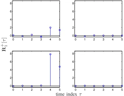
![Fig. 5. Diagonalized CSD matrix D2[τ] generated using the SBR2 algorithm(trimmed as the same order as R2[τ]).](https://thumb-us.123doks.com/thumbv2/123dok_us/1567025.109285/5.595.67.265.309.461/fig-diagonalized-matrix-generated-using-algorithm-trimmed-order.webp)
