An Equivalence Between Adaptive Dynamic Programming With a Critic and Backpropagation Through Time

City, University of London Institutional Repository

Citation:

Fairbank, M., Alonso, E. and Prokhorov, D. (2013). An Equivalence Between

Adaptive Dynamic Programming With a Critic and Backpropagation Through Time. IEEE

Transactions on Neural Networks and Learning Systems, 24(12), pp. 2088-2100. doi:

10.1109/TNNLS.2013.2271778

This is the accepted version of the paper.

This version of the publication may differ from the final published

version.

Permanent repository link:

http://openaccess.city.ac.uk/5184/

Link to published version:

http://dx.doi.org/10.1109/TNNLS.2013.2271778

Copyright and reuse: City Research Online aims to make research

outputs of City, University of London available to a wider audience.

Copyright and Moral Rights remain with the author(s) and/or copyright

holders. URLs from City Research Online may be freely distributed and

linked to.

An Equivalence between Adaptive Dynamic

Programming with a Critic and Backpropagation

Through Time

Michael Fairbank,

Student Member, IEEE

, Eduardo Alonso and Danil Prokhorov,

Senior Member, IEEE

(To appear inIEEE Transactions on Neural Networks and Learning Systems, Vol.??, Issue ??, October 201?, pages ?–?. Copyright the authors and IEEE, http://ieeexplore.ieee.org.)

Abstract—We consider the adaptive dynamic programming technique called Dual Heuristic Programming (DHP), which is designed to learn a critic function, when using learned model functions of the environment. DHP is designed for optimising control problems in large and continuous state spaces.

We extend DHP into a new algorithm that we call VGL(λ), and prove equivalence of an instance of the new algorithm to backpropagation through time for control with a greedy policy. Not only does this equivalence provide a link between these two different approaches, but it also enables our variant of DHP to have guaranteed convergence, under certain smoothness conditions and a greedy policy, when using a general smooth non-linear function approximator for the critic.

We consider several experimental scenarios including some which prove divergence of DHP under a greedy policy, which contrasts against our proven-convergent algorithm.

Index Terms—Adaptive Dynamic Programming, Dual Heuris-tic Programming, Value-Gradient Learning, Backpropagation Through Time, Neural Networks

I. INTRODUCTION

A

DAPTIVE Dynamic Programming (ADP) [1] is the study

of how an agent can learn actions that minimise a long-term cost function. For example a typical scenario is an agent moving in a state space, _S ⊂ _Rn_{, such that at time t it has} state vector ~xt. At each time t ∈ Z+ the agent chooses an action~ut from an action space A, which takes it to the next state according to the environment’s model function

~

xt+1=f(~xt, ~ut), (1)

and gives it an immediate cost or utility, Ut, given by the functionUt=U(~xt, ~ut). The agent keeps moving, forming a trajectory of states(~x0, ~x1, . . .), which terminates if and when a state from the set of terminal states T ⊂ S is reached. If a terminal state ~xt ∈Tis reached then a final instantaneous costUt=U(~xt)is given which is independent of any action. An action network, A(~x, ~z), is the output of a smooth approximated function, e.g. the output of a neural network with parameter vector ~z. The action network, which is also known as the actoror policy, assigns an action

~

ut=A(~xt, ~z) (2)

M. Fairbank and E. Alonso are with the Department of Computer Sci-ence, School of Informatics, City University London, London, UK (e-mail: [email protected]; [email protected]).

D. Prokhorov is with Toyota Research Institute NA, Ann Arbor, Michigan (e-mail: [email protected]).

to take for any given state~xt.

For a trajectory starting from ~x0 derived by following (1) and (2), the total trajectory cost is given by the cost-to-go

function, orvalue function, which is

J(~x0, ~z) =

* X

t

γtU(~xt, ~ut) +

.

Here hi denotes expectation, and γ ∈ [0,1] is a constant

discount factorthat specifies the importance of long term costs over short term ones. The objective of ADP is to train the action network such thatJ(~x0, ~z)is minimised from any~x0. ADP also uses a second approximated function, the scalar valuedcritic network,Je(~x, ~w). This is the output of a smooth general scalar function approximator, e.g. a neural network with a single output node and weight vectorw~. The objective of training the critic network is for it act as a good approxima-tion of the cost-to-go funcapproxima-tion, i.e. so thatJe(~x, ~w)≈J(~x, ~z) for all states~x.

For any given critic network, thegreedy policy is a policy which always chooses actions that lead to states that the critic function rates as best (whilst also taking into account the immediate short term utility in getting there), i.e. a greedy policy chooses actions according to

~u= arg min

~ u∈A

D

U(~x, ~u) +γJe(f(~x, ~u), ~w) E

∀~x. (3) When a critic and action network are used together, the objective is to train the action network to be greedy with respect to the critic (i.e. the action network must choose actions ~ut=A(~xt, ~z) that satisfy (3)), and to train the critic to approximate the cost-to-go function for the current action network. If these two objectives can be met simultaneously, and exactly, for all states, then Bellman’s Optimality Condition [2] will be satisfied, and the ADP objective of optimising the cost-to-go function from any start state will be achieved.

We follow the methods of Dual Heuristic Programming (DHP) and Globalized DHP (GDHP) [1], [3]–[6]. DHP and GDHP work by explicitly learning the gradient of the cost-to-go function with respect to the state vector, i.e. they learn ∂J_∂~x instead ofJ directly. We refer to these methods collectively as

We extend the VGL methods to include a bootstrapping parameterλto give the algorithm we call VGL(λ) [7], [8]. This is directly analogous to how the reinforcement learning (RL) algorithm TD(λ) is extended from TD(0) [9]. This extension

was desirable because, for example, choosing λ = 1 can

lead to increased stability in learning, and guaranteeing stably convergent algorithms is a serious issue for all critic learning algorithms. Also, setting a high value of λ can increase the “look-ahead” of the training process for the critic, which can lead to faster learning in long trajectories.

The VGL methods work very efficiently in continuous do-mains such as autopilot landing [4], power system control [10], simple control benchmark problems such as “pole balancing” [11], and many others [1]. It turns out to be only necessary to learn the value gradient along a single trajectory, while also satisfying the greedy policy condition, for the trajectory to be locally extremal, and often locally optimal. This is for reasons closely related to Pontryagin’s minimum principle [12], as proven by [13]. This is a significant efficiency gain for the VGL methods and is their principal motivation. In contrast, value-learning methods must learn the values all along the trajectory and over all neighbouring trajectories too to achieve the same level of assurance of local optimality [14].

All VGL methods are model-based methods. We assume the functions f andU each consist of a differentiable part plus, optionally, an additive noise part, and we assume they can be learned by a separate “system identification” learning process, for example as described by [15]. This system identification process could have taken place prior to the main learning process, or concurrently with it. From now on in this paper, we assumef(~x, ~u)andU(~x, ~u)refer to the learned, differentiable model functions; and it is with respect to these two learned functions that we are seeking to find optimal solutions. Using a neural network to learn these two functions would enforce the required smoothness conditions onto these two functions. Proving convergence of ADP algorithms is a challenging problem. References [5], [16], [17] show the ADP process will converge to optimal behaviour if the critic could be perfectly learned over all of state space at each iteration. However in reality we must work with a function approximator for the critic with finite capabilities, so this assumption is not valid. Variants of DHP are proven to converge by [18], [19], the first of which uses a linear function approximator for the critic which can be fully trained in a single step, and the second of which is based on the Galerkin-based form of DHP [20], [21]. We do not consider the Galerkin-based methods (which

are also known as residual-gradient methods by [21]) for

reasons given by [22] and [7, sec 2.3]. Working with a general quadratic function approximator, [20, sec.7.7-7.8] proves the general instability of DHP and GDHP. This analysis was for a fixed action network, so with a greedy policy convergence would presumably seem even less likely. In this paper, we show a specific divergence example for DHP with a greedy policy in Section IV.

One reason that the convergence of these methods is dif-ficult to assure is that in the Bellman condition, there is an interdependence between J(~x, ~z), A(x, ~~ z) and Je(~x, ~w). We make an important insight into this difficulty by showing (in

Lemma 4) that the dependency of a greedy policy on the critic is primarily through the value-gradient.

In this paper, using a method first described in our earlier technical reports [7], [13], we show the VGL(λ) weight update, withλ= 1 and some learning constants chosen carefully, is identical to the application of backpropagation through time (BPTT) [23] to a greedy policy. This makes a theoretical con-nection between two seemingly different learning paradigms, and provides a convergence proof for a critic learning ADP method, with a general smooth function approximator and a greedy policy.

In the rest of this paper, in Section II we define the VGL(λ) algorithm, state its relationship to DHP, and give pseudocode for it. Section III is the main contribution of this paper, in which we describe BPTT and the circumstances of its equivalence to VGL(λ) with a greedy policy, and we describe how this equivalence forms a convergence proof for VGL(λ) under these circumstances. In Section IV, we provide an example ADP problem which we use to make a confirmation of the equivalence proof, and which we also use to demonstrate how critic learning methods with a greedy policy can be made to diverge; in contrast to the proven convergent algorithm. In Section V we describe two neural-network based experiments, and give conclusions in Section VI.

II. THEVGL(λ)ANDDHP ALGORITHMS

All VGL algorithms, including DHP, GDHP and VGL(λ),

attempt to learn the value-gradient, ∂J_∂~x. This gradient is learned by a vector critic function Ge(~x, ~w) which has the same dimension asdim(~x). In the case of DHP this function is implemented by the output of a smooth vector function approximator, and in GDHP it is implemented as Ge(~x, ~w)≡

∂Je(~x, ~w)

∂~x , i.e. the actual gradient of the smooth approximated scalar function Je(~x, ~w). For the VGL(λ) algorithm, we can use either of these two representations forGe.

We assume the action networkA(~x, ~z)is differentiable with respect to all of its arguments, and similar differentiability conditions apply to the model and cost functions.

Throughout this paper, subscripted t variables attached to a function name indicates that all arguments of the function are to be evaluated at time steptof a trajectory. This is what we call trajectory shorthand notation. For example Jet+1 ≡

e

J(~xt+1, ~w),Ut≡U(~xt, ~ut)andGet≡Ge(~xt, ~w).

A convention is also used that all defined vector quantities are columns, whether they are coordinates, or derivatives with respect to coordinates. For example, both ~xt and ∂_∂~J_xe are columns. Also any vector function becomes transposed (be-coming a row) if it appears in the numerator of a differential. For example ∂f_∂~x is a matrix with element (i, j) equal to

∂f(~x,~u)j

∂~xi ;

∂Ge

∂ ~w is a matrix with element (i, j) equal to ∂Gej

∂ ~wi;

and∂Ge

∂ ~w

t is the matrix ∂Ge

∂ ~w evaluated at (~xt, ~w). This is the transpose of the common convention for Jacobians.

Using the above notation and implied matrix products, the VGL(λ) algorithm is defined to be a weight update of the form:

∆w~ =αX

t

∂Ge

∂ ~w

!

t

where α is a small positive learning rate; Ωt is an arbitrary positive definite matrix described further below; Get is the output of the vector critic at time stept; andG0tis the “target value gradient” defined recursively by:

G0t=

(

DU D~x

t+γ Df D~x

t

λG0t+1+ (1−λ)Gte+1

if~xt∈/T

∂U ∂~x

t if~xt∈T

(5)

whereλ∈[0,1]is a fixed constant, analogous to the λused in TD(λ); and where _D~D_x is shorthand for

D D~x≡

∂ ∂~x+

∂A ∂~x

∂

∂~u; (6)

and where all of these derivatives are assumed to exist. All terms of (5) are obtainable from knowledge of the model functions and the action network. We ensure the recursion in (5) converges by requiring that either γ < 1, or λ < 1, or the environment is such that the agent is guaranteed to reach a terminal state at some finite time (i.e. the environment is “episodic”).

The objective of the weight update is to make the values

e

Gt move towards the target values G0t. This weight update needs to be done slowly because the targets G0 are heavily dependent on w~, so are moving targets. This dependency on

~

w is especially great if the policy is greedy or if the action network is concurrently trained to try to keep the trajectory greedy, so that the policy is then also indirectly dependent on

~

w. If the weight update succeeds in achievingGet=G0t, and the greedy action condition (3), for all t along a trajectory, then this will ensure the trajectory is locally extremal, and often locally optimal (as proven by [13]).

The matrix Ωt was introduced by Werbos in the GDHP

algorithm (e.g. [20, eq.32]), and is included in our weight update for full generality. This positive definite matrix can be set as required by the experimenter since its presence ensures every component ofGet will move towards the corresponding component of G0t (in any basis). For simplicity Ωt is often just taken to be the identity matrix for allt, so effectively has an optional presence. One use for making Ωt arbitrary could be for the experimenter to be able to compensate explicitly for any rescalings of the state space axes. We make use of it in Section III, when proving how VGL(λ) can be equivalent to BPTT.

Equations (4), (5) and (6) define the VGL(λ) algorithm. Algorithm 1 gives pseudocode for it in a form that can be applied to complete trajectories. This algorithm runs in time

O(dim(w~))per time step of the trajectory. An on-line version is also possible that can be applied to incomplete trajectories [8].

The algorithm does not attempt to learn the value gradient at the final time-step of a trajectory since it is prior knowledge that the target value gradient is always ∂U_∂~x at any terminal state. Hence we assume the function approximator forGe(~x, ~w) has been designed to explicitly return ∂U_∂~x for all terminal states

~ x∈T.

A. Relationship of the VGL(λ) Algorithm to DHP and GDHP

The VGL(λ) algorithm is an extension of the DHP

al-gorithm, made by introducing a λ parameter as defined in

Algorithm 1 VGL(λ). Batch-mode implementation for

episodic environments.

1: t←0

2: {Unroll trajectory...}

3: while not terminated(~xt)do 4: ~ut←A(~xt, ~z)

5: ~xt+1←f(~xt, ~ut)

6: t←t+ 1

7: end while

8: tf ←t 9: ~p← ∂U

∂~x

t,∆w~ ←~0,∆~z←~0 10: {Backwards pass...}

11: fort=tf−1 to0step −1 do 12: G0t← ∂U_∂~x

t+γ

∂f ∂~x

t

~ p

+ ∂A_∂~x t

∂U ∂~u

t+γ _∂f

∂~u

t~p

13: ∆w~ ←∆w~ +∂Ge

∂ ~w

tΩt

G0t−Get

14: ∆~z←∆~z− ∂A ∂~z

t

∂U ∂~u

t+γ

∂f ∂~u

t e

Gt+1

15: ~p←λG0t+ (1−λ)Get 16: end for

17: w~ ←w~+α∆w~

18: ~z←~z+β∆~z

(5). This λ parameter affects the exponential decay rate of the look-ahead used in (5). In this equation, when λ = 0, the target value gradientG0 _{becomes equivalent to the target}

used in DHP. Hence when λ = 0, and when Ge(~x, ~w) is implemented as the vector output of a function approximator, VGL(λ) becomes identical to DHP.

When VGL(λ) is implemented withλ= 0andGe(~x, ~w) is defined to be ∂Je

∂~x, for a scalar function approximatorJe(~x, ~w), it becomes equivalent to an instance of GDHP. GDHP is more general than VGL(0) since its weight update is defined to also include a value-learning component too, i.e. GDHP is a linear combination of the VGL(0) weight update plus a Heuristic Dynamic Programming ( [3], [4]) weight update.

B. Action Network Weight Update

To solve the ADP problem, the action network also needs training. The objective of the action network’s weight update is to make the actor more greedy, i.e. to behave more closely to the following objective:

~

u= arg min

~ u∈A

(Qe(~x, ~u, ~w)) ∀~x (7) where we define the approximate Q Value function as

e

Q(~x, ~u, ~w) =U(~x, ~u) +γJe(f(~x, ~u), ~w), (8)

and which is consistent with (3).

Hence the actor weight update used most commonly in ADP is gradient descent on theQefunction with respect to~z. This is implemented by lines 14 and 18 of Algorithm 1. Hereβ >0

is a separate learning rate for the action network.

can consist of alternating phases of one or more actor weight updates followed by one or more critic weight updates.

C. Greedy Policy

In some implementations the action network can be effi-ciently replaced by a greedy policy, which is a function that directly solves (7). Since the greedy policy (7) is dependent on the weight vector w~ of the critic function, we will denote it as π(~x, ~w)to distinguish it from a general action network

A(~x, ~z). When a greedy policy is used, all occurrences of

A(~x, ~z) in the VGL(λ) algorithm would be replaced by

π(~x, ~w), and the actor weight update equation lines 14 and 18 of Algorithm 1 would be removed.

A greedy policy is only possible when the right-hand side of (7) is efficient to compute, which is possible in the continuous time situations described by [24] or [7, section 2.2], and in the “single network adaptive critic” described by [18]. We give an example of this kind of greedy policy in Section V-B.

D. The Relationship of an Action Network to a Greedy Policy

The main results of this paper apply to a greedy policy: convergence is proven for a greedy policy (in Section III), and so is the divergence of other algorithms (in Section IV). However in certain circumstances, these results can partially apply to an action network too. Since the action network’s weight update is gradient descent on (8), the intention of it is to make the action network behave more like a greedy policy. Hence when the action network is trained to completion in between every single critic weight update (a situation known as value-iteration), then the action network will be behaving very much like a greedy policy. Hence, if the action network has sufficient flexibility to learn the greedy policy accurately enough, then the convergence/divergence results of this paper would apply to it.

III. THERELATIONSHIP OFVGLTOBPTT

We now prove that the VGL(λ) weight update of (4), with

λ = 1 and a carefully chosen Ωt matrix, is equivalent to backpropagation through time (BPTT) on a greedy policy. First we derive the equations for BPTT (in Section III-A), then we describe some lemmas about a greedy policy (in Section III-B), and then we demonstrate that when BPTT is applied to a greedy policy, the weight update obtained is an instance of VGL(λ) (in Section III-C). Finally, in Section III-D, we discuss the consequences of the results and the convergence properties.

A. Backpropagation Through Time for Control Problems

BPTT can be used to calculate the derivatives of any differentiable scalar function with respect the weights of a neural network. To apply BPTT in solving a control problem, it can be used to find the derivatives of J(~x0, ~z)with respect to~z, so as to enable gradient descent on J.

Hence the gradient-descent weight update is ∆~z =

−α ∂J_∂~z0 for some small positive learning rate α. Gradient descent will naturally find local minima of J(~x0, ~z), and has

good convergence properties when the surface J(~x0, ~z) is smooth with respect to~z.

The total discounted cost for a trajectory J(~x0, ~z) =

P tγ

t_U

tcan be written recursively as

J(~x, ~z) =U(~x, A(~x, ~z)) +γJ(f(~x, A(~x, ~z)), ~z) (9)

withJ(~x, ~z) =U(~x)at any terminal state~x∈T.

To calculate the gradient of (9) with respect to ~z, we differentiate using the chain rule, and substitute (1) and (2):

_∂J

∂~z

t

=

_∂

∂~z(U(~x, A(~x, ~z)) +γJ(f(~x, A(~x, ~z)), ~z))

t

=

_∂A

∂~z

t

_∂U

∂~u

t

+γ

_∂f

∂~u

t

_∂J

∂~x

t+1

!

+γ

_∂J

∂~z

t+1

Expanding this recursion and substituting it into the gradient-descent equation gives,

∆~z=−αX

t≥0

γt

_∂A

∂~z

t

_∂U

∂~u

t

+γ

_∂f

∂~u

t

_∂J

∂~x

t+1

!

(10)

This weight update is BPTT with gradient-descent to min-imiseJ(~x0, ~z)with respect to the weight vector~zof an action network A(~x, ~z). It refers to the quantity ∂J_∂~x which can be found recursively by differentiating (9) and using the chain rule, giving

_∂J

∂~x

t

= ( _DU

D~x

t+γ

Df D~x

t ∂J ∂~x

t+1 if~xt∈/ T

∂U ∂~x

t if~xt∈T.

(11)

Equation (11) can be understood to be backpropagating the quantity ∂J_∂~xt+1 through the action network, model and cost functions to obtain ∂J_∂~x

t, and giving the BPTT algorithm its name.

By comparing (11) with (5), we note that

G0≡ ∂J

∂~x, when λ= 1. (12)

B. Lemmas about a Greedy Policy and Greedy Actions

To prepare for the later analysis of BPTT applied to a greedy policy, first we prove some lemmas about the greedy policy. These lemmas apply when the action space, A, is equal to Rdim(~u), which we will denote asA∗.

A greedy policy π(~x, ~w) is a policy that always selects

actions ~u that are the minimum of the smooth function

e

Q(~x, ~u, ~w)defined by (8). These minimising actions are what

we call greedy actions. In this case, since the minimum

of a smooth function is found from an unbound domain,

~

u∈Rdim(~u), the following two consequences hold:

Lemma 1: For a greedy action~uchosen from_A∗, we have ∂Qe

∂~u =~0.

Lemma 2: For a greedy action~uchosen fromA∗, ∂ 2

e

Q ∂~u∂~u is a positive semi-definite matrix.

We now prove too less obvious lemmas about a greedy policy:

Lemma 3: The greedy policy on A∗ implies ∂U∂~u

t =

−γ∂f_∂~u

tGet+1.

Proof: First, we note that differentiating (8) gives

∂Qe

∂~u ! t = ∂U ∂~u t +γ ∂f ∂~u t e

Gt+1 (13)

Substituting this into Lemma 1 and solving for ∂U_∂~u completes the proof.

Lemma 4: When ∂π_{∂ ~wt} and ∂2Qe

∂~u∂~u −1

t exist, the greedy policy on _A∗ implies

∂π ∂ ~w

t

=−γ ∂Ge ∂ ~w

! t+1 ∂f ∂~u T t

∂2Qe

∂~u∂~u

!−1

t

Proof: We use implicit differentiation. The dependency of ~ut = π(x~t, ~w) on w~ must be such that Lemma 1 is always satisfied, since the policy is greedy. This means that _∂ e Q ∂~u t ≡

~_{0, both before and after any infinitesimal change}

to w~. Therefore the greedy policy function π(~xt, ~w)must be such that,

~_{0 =} ∂ ∂ ~w

∂Qe(~xt, π(~xt, ~w), ~w)

∂~ut

!

= ∂

∂ ~w

∂Qe(~xt, ~ut, ~w)

∂~ut !

+

∂π ∂ ~w

t

∂ ∂~ut

∂Qe(~xt, ~ut, ~w)

∂~ut !

= ∂

∂ ~w

_∂U ∂~u t +γ _∂f ∂~u t e

Gt+1

+

_∂π

∂ ~w

t

∂2

e

Q ∂~u∂~u

!

t

= ∂

∂ ~w

_∂U

∂~u

t

+γX

i

_∂(f)i

∂~u

t

(Get+1)i

!

+

_∂π

∂ ~w

t

∂2

e

Q ∂~u∂~u

!

t

=γX

i

_∂(f)i

∂~u

t

∂(Get+1)i

∂ ~w +

_∂π

∂ ~w

t

∂2

e

Q ∂~u∂~u

!

t

=γ ∂Ge ∂ ~w

! t+1 _∂f ∂~u T t + _∂π

∂ ~w

t

∂2

e

Q ∂~u∂~u

!

t

In the above six lines of algebra, the sum of the two partial derivatives in line 2 follows by the chain rule from the total derivative in line 1, since w~ appears twice in line 1. This step has also made use of ~ut =π(~xt, ~w). Also note that the first term in line 2 is not zero, despite the greedy policy’s requirement for ∂Qe

∂~u ≡0, since in this term the~uand w~ are now treated as independent variables. Then in the remaining lines, line 3 is by (13); line 4 just expands an inner product; line 5 follows since ∂U_∂~u and ∂f_∂~u are not functions ofw~; and line 6 just forms an inner product.

Then solving the final line for _{∂ ~}∂π_wtproves the lemma.

C. The equivalence of VGL(1) to BPTT

In Section III-A, the equation for gradient descent on

J(~x, ~z)was found for a general policyA(~x, ~z), using BPTT. But BPTT can be applied to any policy, and so we now consider what would happen if BPTT is applied to the greedy policy π(~x, ~w), with actions chosen from A∗. The parameter vector for the greedy policy is w~. Hence we can do gradient descent with respect to w~ instead of~z (assuming the deriva-tives ∂π_{∂ ~w} and _{∂ ~}∂J_w exist). We should emphasise that with the greedy policy, it is the same weight vector that appears in the critic, w~, as appears in the greedy policyπ(~x, ~w).

Consequently, for the gradient-descent equation in BPTT for control (10), we now change all instances ofA and~z to

πandw~, respectively, giving the new weight update:

∆w~ =−αX

t≥0

γt

_∂π

∂ ~w

t _∂U ∂~u t +γ _∂f ∂~u t _∂J ∂~x t+1 !

Substituting Lemmas 3 and 4, and ∂J_∂~xt≡G0twithλ= 1 (by (12)), into this gives:

∆w~ =−αX

t≥0

γt



−γ2

∂Ge

∂ ~w

! t+1 _∂f ∂~u T t ∂2 e Q ∂~u∂~u

!−1

t

_∂f

∂~u

t

(−Get+1+G0t+1)

=αX

t≥0

γt+1 ∂Ge ∂ ~w

!

t

Ωt(G0t−Get) (14) where

Ωt=    ∂f ∂~u T

t−1

∂2Qe

∂~u∂~u −1

t−1

∂f ∂~u

t−1 for

t >0

0 fort= 0

, (15)

and is positive semi-definite, by the greedy policy (Lemma 2). Equation (14) is identical to a VGL weight update equation (4), with a carefully chosen matrix for Ωt, and γ =λ = 1, provided _{∂ ~}∂π_wt and

∂2Qe

∂~u∂~u −1

t exist for all

t. If _{∂ ~}∂π_wtdoes not exist, then _{∂ ~}∂J_w is not defined either.

This completes the demonstration of the equivalence of a critic learning algorithm (VGL(1), with the conditions stated above) to BPTT (with a greedy policy with actions chosen fromA∗, and when ∂ ~∂Jw exists).

Furthermore, the presence of theγtfactor in (14) could be removed if we changed the BPTT gradient-descent equation by removing theγt_{factor from (10). This would make the BPTT} weight update more accurately follow the spirit and intention of the on-line critic weight update; and then the equivalence

of VGL(1) to BPTT would hold for anyγ too.

D. Discussion

BPTT is gradient descent on a function which is bounded below. Therefore, assuming the surface of J(~x, ~z)in~z-space is sufficiently smooth and the step-size for gradient descent is sufficiently small, convergence of BPTT is guaranteed.

good convergence guarantees of BPTT will apply to VGL(1) (when used with the special choice of Ωt by (15)). In this case, this particular VGL algorithm will achieve monotonic

progress with respect to J, and so will have guaranteed

convergence, provided it is operating within a smooth region of the surface of the functionJ. Significantly, the requirement for

∂π

∂ ~w to always exist is satisfied when a value-gradient greedy-policy, of the kind used in our experiments in Section V-B, is used. The requirement for the surface of J in ~z-space to be sufficiently smooth cannot so easily be guaranteed, but this situation is no different than the requirement for BPTT.

This equivalence result was surprising to the authors be-cause it was thought that the VGL weight updates (equation (4), and DHP and GDHP) were based on gradient descent on

an error function E =P

t(G

0

t−Get)TΩt(G0t−Get). But as [21] showed, the TD(λ) weight update is not true gradient descent on its intended error function, and furthermore it is not gradient descent on any error function [25]. Similarly, nor is the VGL(λ) weight update true gradient descent on

E (unless both the policy is fixed and λ = 1). Our proof shows that when a greedy policy is used, VGL(1) is closer to true gradient descent onJ than the gradient onE. It was also surprising to learn that BPTT and critic weight updates are not as fundamentally different to each other as we first thought.

For a fuller discussion of the Ωt matrix defined by (15), including methods for its computation and a discussion of its purpose and effectiveness, see reference [26].

IV. EXAMPLEANALYTICALPROBLEM

In this section we define an ADP problem which is simple enough to analyse algebraically. We define this problem and derive the VGL(λ) weight update algebraically for it in sec-tions IV-A to IV-F. Then in Section IV-G we show that when the Ωt matrix of (15) is used, we do get exact equivalence of VGL(1) to BPTT in the example problem, thus confirming the theoretical result of Section III. We also use the example problem to derive divergence instances for DHP and VGL(λ) without the specialΩtmatrices (in sections IV-H to IV-I), thus emphasising the value of the BPTT equivalence proof.

A. Environment Definition

We define an environment with state x ∈ R and action

u∈R, and with model and cost functions:

f(xt, t, ut) =xt+ut for t∈ {0,1} (16a)

U(xt, t, ut) =k(ut)2 for t∈ {0,1} (16b) where k > 0 is a constant. Each trajectory is defined to terminate immediately on arriving at time stept= 2, when a final terminal cost of

U(xt) = (xt)2 (17)

is given, so that exactly three costs are received by the agent over the full trajectory duration. The termination condition is dependent on t, so strictly speaking t should be included in the state vector, but we have omitted this for brevity.

A whole trajectory is completely parametrised by x0, u0 andu1, and the total cost is

J =k(u0)2+k(u1)2+ (x0+u0+u1)2. (18) The examples we derive below consider a trajectory which starts atx0= 0. From this start point, the optimal actions are those that minimiseJ, i.e.u0=u1= 0.

B. Critic Definition

A critic function is defined using a weight vector with just two weights,w~ = (w1, w2)T:

e

J(xt, t, ~w) =   

 

0 if t= 0

c1(x1)2−w1x1 if t= 1

c2(x2)2−w2x2 if t= 2

(19)

wherec1 andc2 are positive constants. These two constants are not to be treated as weights. We included them so that we could consider a greater range of function approximators for the critic when we searched for a divergence example, as described in Section IV-H. Also to ease the finding of that divergence example, we chose this simplified critic structure (as opposed to a neural network) since it is linear inw~, and its weight vector has just two components.

Hence the critic gradient function,Ge≡∂_∂xJe, is given by:

e

G(xt, t, ~w) = (

0 ift= 0

2ctxt−wt ift∈ {1,2}

(20)

We note that this implies

∂Ge

∂wk !

t

= (

−1 ift∈ {1,2} andt=k

0 otherwise (21)

C. Unrolling a greedy trajectory

Agreedy trajectoryis a trajectory that is found by following greedy actions only. Greedy actions are~uvalues that minimise

e

Q(~x, ~u, ~w).

Substituting the model functions (16) and the critic defini-tion (19) into theQefunction definition (8) gives, withγ= 1,

e

Q(xt, t, ut, ~w)

=U(xt, t, ut) +γJ(f(xt, t, ut), te + 1, ~w) by (8)

=k(ut)2+J(xte +ut, t+ 1, ~w), fort∈ {0,1} by (16)

=

(

k(u0)2+c1(x0+u0)2−w1(x0+u0) ift= 0

k(u1)2+c2(x1+u1)2−w2(x1+u1) ift= 1

by (19)

=k(ut)2+ct+1(xt+ut)2−wt+1(xt+ut), fort∈ {0,1}. In order to minimise this with respect tout and get greedy actions, we first differentiate to get,

∂Qe

∂u

!

t

= 2kut+ 2ct+1(xt+ut)−wt+1 fort∈ {0,1}

= 2ut(ct+1+k)−wt+1+ 2ct+1xt fort∈ {0,1}

(22)

Hence the greedy actions are found by solving ∂Qe

∂u

t

= 0, to obtain,

u0≡

w1−2c1x0

2(c1+k)

u1≡

w2−2c2x1

2(c2+k)

(24)

and these two equations define the greedy policy function

π(~x, ~w)for this environment and critic function.

Since the optimal actions areu0=u1= 0from a start state of x0= 0, the optimal weights arew1=w2= 0.

Following the greedy actions along a trajectory starting at

x0 = 0, and using the recursion xt+1 = f(xt, ut) with the model functions (16) gives

x1=x0+u0 by (16a)

= w1

2(c1+k)

by (23) &x0= 0, (25)

and,

x2=x1+u1 by (16a)

= w2(c1+k) +kw1 2(c2+k)(c1+k)

. by (24) & (25). (26)

Substitutingx1(25) back into the equation foru1(24) gives

u1 purely in terms of the weights and constants:

u1≡

w2(c1+k)−c2w1

2(c2+k)(c1+k)

(27)

D. Evaluation of value-gradients along the greedy trajectory

We can now evaluate theGevalues by substituting the greedy trajectory’s state vectors (eqs. (25)-(26)) into (20), giving:

e

G1= 2c1x1−w1 by (20)

= c1w1 (c1+k)

−w1 by (25)

= −w1k (c1+k)

(28)

and

e

G2= 2c2x2−w2 by (20)

= w2(c1+k)c2+kw1c2 (c2+k)(c1+k)

−w2 by (26)

= kw1c2−w2k(c1+k) (c2+k)(c1+k)

. (29)

The greedy actions of equations (23) and (24) both satisfy

_∂π

∂x

t

= −ct+1

ct+1+k

for t∈ {0,1} (30)

Substituting (30) and (16a) into the definition forDf_Dx tgiven by (6), gives,

_Df

Dx

t

=

_∂f

∂x

t

+

_∂π

∂x

t

_∂f

∂u

t

by (6)

=

_∂x+u

∂x

t

+

_∂π

∂x

t

_∂x+u

∂u

t

by (16a)

= 1− ct+1

ct+1+k

, fort∈ {0,1} by (30)

= k

ct+1+k

, for t∈ {0,1}. (31)

Similarly, the expression for DU_Dxt is found by:

_DU

Dx

t

=

_∂U

∂x

t

+

_∂π

∂x

t

_∂U

∂u

t

by (6)

=

_∂k(u)2

∂x

t

+

_∂π

∂x

t

_∂k(u)2

∂u

t

by (16b)

= 0− ct+1

ct+1+k

(2kut), for t∈ {0,1} by (30)

=−2kct+1ut

ct+1+k

, for t∈ {0,1}. (32)

E. Backwards pass along trajectory

We do a backwards pass along the trajectory calculating the target gradients using (5) withγ= 1:

G02=

_∂U

∂x

2

by (5) with x2∈T

=2x2 by (17)

=w2(c1+k) +kw1 (c2+k)(c1+k)

by (26) (33)

Similarly,

G01=

_DU

Dx

1

+

_Df

Dx

1

λG02+ (1−λ)Ge2

by (5)

=−2kc2u1

c2+k

+ k

c2+k

λG02+ (1−λ)Ge2

by (32),(31)

=−kc2(w2(c1+k)−c2w1) (c1+k)(c2+k)2

by (27)

+ k

c2+k

λw2(c1+k) +kw1

(c2+k)(c1+k)

by (33)

+(1−λ)kw1c2−w2k(c1+k) (c2+k)(c1+k)

by (29)

=w1k(kλ+ (c2)

2_+k(1−λ)c 2)

(c1+k)(c2+k)2

−w2k(c2−λ+k(1−λ))

(c2+k)2

(34)

F. Analysis of weight update equation

We now have the whole trajectory and the termsGe andG0 written algebraically, so that we can next analyse the VGL(λ) weight update algebraically.

The VGL(λ) weight update (4) is comprised of

X

t

∂Ge

∂wi !

t

Ωt(G0t−Get)

=−Ωi(G0i−Gei) (fori∈ {1,2}, by (21)). Switching to vector notation forw~, this is

X

t

∂Ge

∂ ~w

!

t

Ωt(G0t−Get) =−

Ω1(G01−Ge1)

Ω2(G02−Ge2)

!

=−

Ω1 0

0 Ω2

G01−Ge1

G02−Ge2

=DB ~w (35)

where

D=

Ω1 0

0 Ω2

(36)

and B is a 2×2 matrix with elements found by subtracting equations (28) and (29) from equations (34) and (33), respec-tively, giving,

B=−

k(kλ+(c2)2+k(1−λ)c2) (c1+k)(c2+k)2 +

k

(c1+k)

−k(c2+k−λ(k+1)) (c2+k)2 k(1−c2)

(c2+k)(c1+k)

1+k

(c2+k)

!

(37)

By equations (4) and (35), ∆w~ = αDB ~w is the VGL(λ) weight update written as a single dynamic system of w~.

G. Equivalence of BPTT to VGLΩ(1) for this Example Prob-lem

We define VGLΩ(λ)to be the VGL(λ) algorithm combined with theΩtmatrix of (15). We now demonstrate that VGLΩ(1) is identical to the BPTT equation derived for this example problem. The purpose of this subsection is just to provide a confirmation of the main equivalence proof of this paper (Section III), in the context of our simple example problem.

To construct theΩtmatrix of (15), we differentiate (22) to get ∂2 e Q ∂u∂u ! t

= 2(ct+1+k) for t∈ {0,1}. (38)

and then substitute (38) and∂f_∂u

t= 1(by (16a)) into (15), to get

Ωt= (

1/(2(ct+k)) for t∈ {1,2}

0 for t= 0.

Substituting these Ωt matrices into the D matrix of (36) gives

D=

1

2(c1+k) 0

0 _2(c1

2+k) !

(39)

The VGLΩ(1)weight update, with α= 1, is

∆w~ =DB ~w by (4), (35)

=−D

k(k+(c2)2)

(c1+k)(c2+k)2 + k

(c1+k)

k(1−c2)

(c2+k)2 k(1−c2)

(c2+k)(c1+k)

1+k

(c2+k)

!

~

w by (37),λ= 1 =−2D

k(k+(c2)2)

(c2+k)2 +k

k(1−c2)

(c2+k) k(1−c2)

(c2+k) 1 +k !

D ~w by (39)

(40)

We aim to show that this equation is identical to gradient descent onJ, i.e.∆w~ =−∂J

∂ ~w. First we consider the equations that determine how the actions u0 andu1 depend on w~. By equations (25) and (27), we have

u0 u1 = 1

2(c1+k) 0

−c2

2(c2+k)(c1+k)

1 2(c2+k)

!

~ w

=ED ~w (41)

whereD is given by (39) and

E= −c1₂ 0 c2 +k 1

. (42)

Now we can consider the gradient descent equation as follows:

−∂J

∂ ~w =−

∂ k(u0)2+k(u1)2+ (x0+u0+u1)2

∂ ~w by (18)

=−2ku0

∂u0

∂ ~w −2ku1 ∂u1

∂ ~w −2(u0+u1)

∂u0

∂ ~w + ∂u1

∂ ~w

=−2((k+ 1)u0+u1)

∂u0

∂ ~w −2(u0+ (k+ 1)u1) ∂u1

∂ ~w =−2∂u0

∂ ~w k+ 1 1

u0

u1

−2∂u1

∂ ~w 1 k+ 1

u0

u1

=−2 ∂u0 ∂w1 ∂u1 ∂w1 ∂u0 ∂w2 ∂u1 ∂w2 !

k+ 1 1 1 k+ 1

u0

u1

=−2DET

k+ 1 1 1 k+ 1

ED ~w by (41)

=−2DET

k+ 1 1 1 k+ 1

1 0 −c2

c2+k 1

D ~w by (42)

=−2D

1 −c2

c2+k 0 1

_k+ k

c2+k 1

k(1−c2)

c2+k k+ 1 !

D ~w by (42)

=−2D

k(k+(c2)2) (c2+k)2 +k

k(1−c2) (c2+k)

k(1−c2)

(c2+k) k+ 1 !

D ~w

This final line is identical to (40), which completes the proof of exact equivalence of VGLΩ(1)to BPTT for this particular problem.

H. Divergence Examples for VGL(0) and VGL(1)

We now show that unlike VGLΩ(1), the algorithms DHP

and VGL(1) can both be made to diverge with a greedy policy in this problem domain.

To add further complexity to the system, in order to achieve the desired divergence, we next definew~ to be a linear function of two other weights,~p= (p1, p2)T, such thatw~ =F ~p, where

F is a2×2 constant real matrix. The VGL(λ) weight update equation can now be recalculated for these new weights, as follows:

∆~p=αX t

∂Ge

∂~p

!

t

Ωt(G0t−Gt)e by (4)

=αX t

∂ ~w ∂~p

∂Ge

∂ ~w

!

t

Ωt(G0t−Gt)e by chain rule

=α∂ ~w ∂~p

X

t ∂Ge

∂ ~w

!

t

Ωt(G0t−Gt)e since independent oft

=α∂ ~w

∂~pDB ~w by (35)

=α(FTDBF)~p. byw~=F ~pand ∂ ~w

∂~p = ∂(F ~p)

∂~p =F T

(43)

Equation (43) represents the whole learning system, de-scribed as a dynamical system of the weight vector ~p.

The optimal actions u0 =u1 = 0 would be achieved by

~

p=~0. To produce a divergence example, we want to ensure that ~pdoes not converge to~0.

Takingα >0to be sufficiently small, then the weight vector

~

p evolves according to a continuous-time linear dynamic

system (equation (43), with D ignored), and this system is stable if and only if the matrix product FT_{BF is “stable”} (i.e. if the real part of every eigenvalue of this matrix product is negative). The logic here is that if it is proven to diverge for a continuous time system, i.e. in the limit of an infinitesimal learning rate, then it would also diverge for any small finite learning rate too.

Choosing λ = 0, with c1 = c2 = k = 0.01 gives

B = ₋−₂₄0._.75₇₅₋0₅₀.5_.5

(by (37)). ChoosingF = 10 1

−1−1

makes

FTBF = ₁₈₉117._.00−₋38₂₇._.25₀which has eigenvalues 45±45.22i. Since the real parts of these eigenvalues are positive, (43) will diverge for VGL(0) (i.e. DHP).

Also, perhaps surprisingly, it is possible to get instability with VGL(1). Choosing c2 = k = 0.01, c1 = 0.99 gives

B = −₋0₀._.2625₄₉₅ −₋24₅₀._.75₅

. Choosing F = −1−1

.2 .02

makes

FT_{BF =} 2.7665 0.1295 4.4954 0.2222

[image:10.612.68.267.369.461.2]

which has two positive real eigen-values. Therefore this VGL(1) system diverges.

Fig. 1 shows the divergences obtained for VGL(0) and VGL(1) with a greedy policy.

1e-10 1e-08 1e-06 0.0001 0.01 1 100 10000

100 ₁₀1 ₁₀2 ₁₀3 ₁₀4 ₁₀5 ₁₀6 ₁₀7

|

~p

|

Iterations VGL(0)/DHP

VGL(1) VGLΩ(1)

Fig. 1. Diverging behaviour for VGL(0) (i.e. DHP) and VGL(1), using the learning parameters described in Section IV-H and a learning rate of

α= 10−6_{); and converging behaviour on the same problem for VGLΩ(1),} as described in Section IV-I, withα= 10−3_.

I. Results for VGLΩ(1) and VGLΩ(0)

VGLΩ(λ) is defined to be VGL(λ) with the Ωt matrix defined by (15). As predicted by the convergence proof of Section III, and the explicit demonstration of Section IV-G,

it was not possible to make the VGLΩ(1) weight update

diverge. An example of VGLΩ(1) converging under the same conditions that caused VGL(1) to diverge is given in Fig.1.

Next, we considered VGLΩ(0). Substituting the same pa-rameters that made VGL(0) diverge, i.e. c1=c2=k= 0.01,

into (39) gives D = 25 0

0 25

. Since D is a positive multiple of the identity matrix, its presence in (43) will not affect the stability of the productFTDBF, so the system for~pwill still be unstable, and diverge, just as it did for VGL(0) (where D

was taken to be the identity matrix). So unfortunately using the Ωtmatrix of (15) does not force reliable convergence for VGL(0) (i.e. DHP) with a greedy policy.

V. NEURAL-NETWORKEXPERIMENTS

To extend the experiments of the previous section that used a quadratic function approximator for the critic, in this section we consider two neural-network based critic experiments: a vertical-spacecraft problem and the cart-pole benchmark problem.

A. Vertical-Spacecraft Problem

A spacecraft of mass m is dropped in a uniform gravita-tional field. The spacecraft is constrained to move in a vertical line, and a single thruster is available to make upward acceler-ations. The state vector of the spacecraft is~x= (h, v, t)T and has three components: height (h), velocity (v) and time step (t). The action vector is one-dimensional (so that~u≡u∈R) producing accelerations u ∈ [0,1]. The Euler method with time-step∆tis used to integrate the equation of motion, giving the model function:

f((h, v, t)T, u) =(h+v∆t, v+ (u−kg)∆t, t+ 1)T Here,kg= 0.2 is a constant giving the acceleration due to gravity (which is less than the range of u; so the spacecraft can overcome gravity easily).∆t was chosen to be 0.4.

A trajectory is defined to last exactly 200 time steps. A final impulse of cost equal to

U(~x) =1 2mv

2_+m(k

g)h (44)

is given on completion of the trajectory. This cost penalises the total kinetic and potential energy that the spacecraft has at the end of the trajectory. This means the task is for the spacecraft to lose as much mechanical energy as possible throughout the duration of the trajectory, to prepare for a gentle landing. The optimal strategy for this task is to leave the thruster switched off for as long as possible in the early stages of the journey, so as to gain as much downward speed as possible and hence lose as much potential energy as possible, and at the end of the journey produce a burst of continuous maximum thrust to reduce the kinetic energy as much as possible.

In addition to the cost received at termination by (44), a cost is also given for each non-terminal step. This cost is

U(~x, u) =c

ln(2−2u)−uln ₁

−u u

∆t (45)

wherec= 0.01is constant. This cost function is designed to ensure that the actions chosen will satisfy u∈[0,1], even if a greedy policy is used. We explain how this cost function was derived, and how it can be used in a greedy policy, in Section V-B, but first we describe experiments that did not use a greedy policy.

MLP, we used a rescaled state vector ~x0 defined to be

~

x0= (h/1600, v/40, t/200)T. In our implementation, we also used redefined model and cost functions that work directly with the rescaled state vectors, i.e. we rescaled them so that

~

x0_t+1 =f(~x0_t, ~ut)andUt=U(~x0t, ~ut). By doing this we also ensured that the output of the neural network, Ge, was also suitably scaled.

The action network was identical in design to the critic, except there was only one output node, and this had a logistic sigmoid function as its activation function. The output of the action network gave the spacecraft’s acceleration udirectly.

The mass of the spacecraft used was m= 0.02. In all of the experiments we made the trajectory always start fromh= 1600, v = −2, and used discount factor γ = 1. The exact derivatives of the functions f(~x, ~u) and U(~x, ~u) were made available to the algorithms.

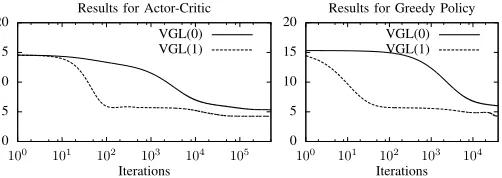
Results using the actor-critic architecture and Algorithm 1 are given in the left-hand graph of Fig. 2, comparing the performance of VGL(1) and VGL(0) (DHP). Each curve shows algorithm performance averaged over 40 trials.

The graphs show that the VGL(1) algorithm produces a lower total costJ than the VGL(0) algorithm does, and does it faster. It is thought that this is because in this problem the major part of the cost comes as a final impulse, so it is advantageous to have a long look-ahead (i.e. a high λvalue) for fast and stable learning.

For the actor-critic learning we chose the learning rate of the actor to be high compared to the learning rate for the critic (i.e.β > α). This was to make the results comparable to those of a greedy policy which we try in the next section.

0 5 10 15 20

100 ₁₀1 ₁₀2 ₁₀3 ₁₀4 ₁₀5 Iterations

Results for Actor-Critic VGL(0) VGL(1)

0 5 10 15 20

100 ₁₀1 ₁₀2 ₁₀3 ₁₀4 Iterations Results for Greedy Policy

[image:11.612.47.298.419.508.2]

VGL(0) VGL(1)

Fig. 2. VGL(0) (i.e. DHP) and VGL(1): The left-hand graph shows Actor-Critic performance, using learning ratesα= 10−6_{andβ= 0.01as described} in Section V-A; and the right-hand graph shows performance with a greedy policy andα= 10−6 _{as described in Section V-B.}

B. Vertical-Spacecraft Problem with Greedy Policy

The cost function of (45) was derived to form an efficient greedy policy, by following the method of [24]. This method uses a continuous time approximation that allows the greedy policy to be derived in the form of an arbitrary sigmoidal functiong(·). To achieve a range ofu∈(0,1), we chosegto be the logistic function,

g(x) = 1

1 +e−x/c. (46)

The choice ofcaffects the sharpness of this sigmoid function. Using this chosen sigmoid function, the cost function based on [24] is defined to be

U(~x, u) = ∆t

Z

g−1(u)du. (47)

Note that solving this integral gives (45). Then to derive the greedy policy for this cost function, we make a first order Taylor series expansion of theQe(~x, ~u, ~w) function (8) about the point~x:

e

Q(~x, ~u, ~w)≈U(~x, ~u) +γ





∂Je

∂~x

!T

(f(~x, ~u)−~x) +J(~ex, ~w) 



=U(~x, ~u) +γG(~ex, ~w) T

(f(~x, ~u)−~x) +γJ(~ex, ~w)

(48)

This approximation becomes exact in continuous time, i.e. in the limit as ∆t → 0. The greedy policy must minimise Qe, hence we differentiate (48) to get

∂Qe

∂u

!

t

=

_∂U

∂u

t

+γ

_∂f

∂u

t e

Gt by (48)

=g−1(ut)∆t+γ

_∂f

∂u

t e

Gt by (47) (49)

For a minimum, we must have ∂Qe

∂u = 0, which, since ∂f ∂u is independent ofu, gives the greedy policy as

π(~xt, ~w) =g

− γ

∆t

_∂f

∂u

t e

Gt

. (50)

We note that this type of greedy policy is very similar to the Single Network Adaptive Critic (SNAC) formulation proposed by [18].

This is the sigmoidal form for the greedy policy that we sought to derive. We used this greedy policy function (50) in place of A(~x, ~z) in lines 4 and 12 of Algorithm 1. For the occurrence of ∂A_∂~x in line 12, we differentiated (50) directly to obtain

_∂π

∂~x

t

=g0

− γ

∆t

_∂f

∂u

t e

Gt

− γ

∆t ∂Ge

∂~x

!

t

_∂f

∂u

T

t !

(51) whereg0(x)is the derivative of the function g(x)and where we have used the fact that for these model functions~uis one-dimensional and _∂~∂_x∂u2f = 0. Lines 14 and 18 of the algorithm were not used.

The results for experiments using the greedy policy are shown in the right-hand graph of Fig. 2. Comparing the left-hand and right-left-hand graphs we see the relative performance between VGL(1) and VGL(0) is similar. This indicates that in this experiment, the greedy policy derived can successfully replace the action network, raising efficiency, and without any apparent detriment.

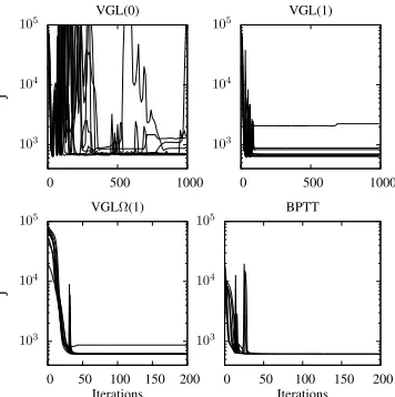
Using a greedy policy, there are no longer two mutually interacting neural networks whose training could be interfering with each other. With the simpler architecture of just one neu-ral network (the critic) to contend with, we attempt to speed up learning using RPROP [27]. Results are shown in the two left-hand graphs of Fig. 3. It seems the aggressive acceleration by RPROP can cause large instability in the VGL(1) and DHP (VGL(0)) algorithms. This is because neither of these two algorithms is true gradient descent when used with a greedy policy (e.g. as shown in Section IV).

However when the Ωt matrix defined by (15) is used

0 5 10 15 20

0 500 1000

J

Iterations VGL(0)

0 5 10 15 20

0 500 1000

Iterations VGL(1)

0 5 10 15 20

0 500 1000

[image:12.612.47.301.51.141.2]

Iterations VGLΩ(1)

Fig. 3. Solution of the spacecraft problem by VGL(0), VGL(1) and VGLΩ(1), with a greedy policy, using RPROP. Each graph shows the performance of a learning algorithm for each of ten different weight initialisations; hence the ensemble of curves in each graph gives some idea of an algorithm’s reliability and volatility.

monotonic progress, as shown in the right-hand graph of Fig. 3, and as explained by the equivalence proof of Section III.

In this case, due to the continuous time approximations made earlier, we modified Ωt from (15) into

Ωt=

_∂f

∂u

T

t

∂2

e

Q ∂u∂u

!−1

t

_∂f

∂u

t

,

with ∂2Qe

∂u∂u found by differentiating (49), giving

∂2

e

Q ∂u∂u

!

t

=

∂g−1_(u

t)∆t+γ _∂f

∂u

tGet

∂ut

by (49)

= ∂g

−1_(u

t)

∂ut

∆t (since ∂

2

f

∂u∂u = 0and ∂Gte

∂ut = 0)

= 1

g0_(g−1_(u

t))

∆t (differentiating an inverse)

= 1

g0₋γ

∆t _∂f

∂u

tGet

∆t by (50)

⇒Ωt=

1 ∆t

_∂f

∂u

T

t

g0

− γ

∆t

_∂f

∂u

t e

Gt

∂f ∂u

t (52)

This equation forΩtis advantageous to use over (15) in that it is always defined to exist (i.e. there is no matrix to invert), it is always positive semi-definite, and it is very efficient to implement. Hence we use (52) in preference to (15) in our experiments here. However (52) is only an approximation to (15), hence the applicability of the equivalence to BPTT proof of III-C will only be approximate; but the approximation

becomes exact in the limit ∆t → 0, and in practice the

empirical results are good with the finite ∆t value that we used, as shown in the right-hand graph of Fig. 3. This graph shows the minimum being reached stably and many times quicker than the other algorithms considered.

Unfortunately, since the value of Ωt given by (52) is not full rank, it does not make a good candidate for use in DHP, or for any VGL(λ) algorithm withλ <1. This is an area for future research.

C. Cart-Pole Experiment

We applied the algorithm to the well known cart-pole benchmark problem described in Fig. 4. The equation of

F θ

x

Fig. 4. Cart-pole benchmark problem. A pole with a pivot at its base is balancing on a cart. The objective is to apply a changing horizontal forceF

to the cart which will move the cart backwards and forwards so as to balance the pole vertically. State variables are pole angle,θ, and cart position,x, plus their derivatives with respect to time,θ˙andx˙.

motion for this system ( [11], [28], [29]), in the absence of friction, is:

¨

θ=

gsinθ−cosθhF+_mmlθ˙2sinθ

c+m i

lh4₃−mcos2_θ mc+m

i (53)

¨

x=

F+mlhθ˙2_sinθ−θ¨_cosθi

mc+m

(54)

where gravitational acceleration, g = 9.8ms−2_{; cart’s mass,}

mc = 1kg; pole’s mass, m = 0.1kg; half pole length,

l = 0.5m; F ∈ [−10,10] is the force applied to the cart, in Newtons; and θ is the pole angle, in radians. The motion was integrated using the Euler method with a time constant

∆t = 0.02, which, for a state vector ~x≡(x, θ,x,˙ θ˙)T, gives a model functionf(~x, ~u) =~x+ ( ˙x,θ,˙ x,¨ θ¨)T∆t.

To achieve the objective of balancing the pole and keeping the cart close to the origin,x= 0, we used a cost function

U(~x, t, u) =γt 5x2+ 50θ2

+c

ln(2−2u)−uln _1−u

u

∆t

(55)

applied at each time step, and the term with coefficient c is there to enable an efficient greedy policy as in Section V-B, but here with c = 10. Each trajectory was defined to last exactly 300 timesteps, i.e. 6 seconds of real time, regardless of whether the pole swung below the horizontal or not, and with no constraint on the magnitude ofx. This cost function and the fixed duration trajectories is similar to that used by [11], [24], but differs to the trajectory termination criterion used by [28] which relies upon a non-differentiable step cost function, and hence is not appropriate for VGL based methods. We used

γ = 0.96 as a discount factor in (55). This discount factor is placed in the definition of U so that the sharp truncation of trajectories terminating after 6 seconds is replaced by a smooth decay. This is preferable to the way that Algorithm 1 implements discount factors, which effectively treats each time step as creating a brand new cost-to-go function to minimise. Following the same derivation as in Section V-B, a greedy

policy was given by (50), which we used to map utoF by

Ft≡20ut−10(to achieve the desired range F ∈[−10,10] when using using g(x) defined by (46)). Again, Ωt and ∂π_∂~x were given by (52) and (51), respectively.

[image:12.612.52.303.275.502.2]

with extra shortcut connections from the input layer to the output layer. The activation functions used were hyperbolic tangent functions at all nodes except for the output layer which used the identity function. Network weights were initially ran-domised uniformly from the range [−0.1,0.1]. To ensure the state vector was suitably scaled for input to the MLP, we used rescaled state vectors~x0defined by~x0= (0.16x,4θ/π,x,˙ 4 ˙θ)T throughout the implementation. As noted by [11], choosing an appropriate state-space scaling was critical to success with DHP on this problem.

Learning took place on 10 trajectories with fixed start points randomly chosen with |x| < 2.4, |θ| < π/15, |x˙| < 5,

|θ˙|<5, which are similar to the starting conditions used by [28]. The exact derivatives of the model and cost functions were made available to the algorithms. Four algorithms were tested and their results are shown in Fig. 5. Both VGL(1) and VGL(0) performed badly when accelerated by RPROP. The results again show that VGLΩ(1) had less volatility and better performance than both VGL(1) and VGL(0), which demonstrates the effectiveness of theΩtmatrix used. For com-parison, we also show the results of an actor-only architecture (i.e. with no critic) trained entirely by BPTT and RPROP. This demonstrates that the minimum attained by the VGL algorithms is suitably low. Also we observed that when this minimum was reached, the pole was being balanced effectively with the cart remaining close to x= 0.

103

104

105

0 500 1000

J

VGL(0)

103

104

105

0 500 1000

VGL(1)

103

104

105

0 50 100 150 200

J

Iterations VGLΩ(1)

103

104

105

0 50 100 150 200

Iterations BPTT

Fig. 5. Cart-pole solutions by VGL(0), VGL(1) and VGLΩ(1), with a greedy policy, plus, for comparison, BPTT. All algorithms were used in conjunction with RPROP. Each graph shows the performance of a learning algorithm for each of ten different random weight initialisations; hence each ensemble of curves gives some idea of an algorithm’s reliability and volatility.

The results show the cart-pole problem being solved effec-tively. We have achieved largely monotonic progress (with the brief non-monotonicity down to the aggressive acceleration of RPROP and/or discontinuities in the cost-to-go function sur-face in weight space) for a critic learning algorithm, replicating the performance of BPTT by a critic with a greedy policy.

VI. CONCLUSIONS

We have found a strong theoretical equivalence between

BPTT and an ADP critic weight update (VGLΩ(1)), two

algorithms that on first sight appeared to be operating totally differently. This provides a convergence proof for this VGL algorithm under the conditions stated in Section III-D. This analysis has been successful for a VGL learning system where a greedy policy is used. Analytical and empirical confirmations of the equivalence to BPTT have been provided in sections IV-G and V, respectively. This contrasts to the demonstrated divergence in Section IV of several other critic algorithms with a greedy policy (DHP, VGL(1) and VGLΩ(0)).

In the experiments of Section V we have shown the effec-tiveness of the algorithm and its ability to produce approximate monotonic learning progress for a neural-network based critic with a greedy policy, even when combined with an aggressive learning accelerator such as RPROP.

REFERENCES

[1] F.-Y. Wang, H. Zhang, and D. Liu, “Adaptive dynamic programming: An introduction,” IEEE Computational Intelligence Magazine, vol. 4, no. 2, pp. 39–47, 2009.

[2] R. E. Bellman,Dynamic Programming. Princeton, NJ, USA: Princeton University Press, 1957.

[3] P. J. Werbos, “Approximating dynamic programming for real-time control and neural modeling.” inHandbook of Intelligent Control, White and Sofge, Eds. New York: Van Nostrand Reinhold, 1992, ch. 13, pp. 493–525.

[4] D. Prokhorov and D. Wunsch, “Adaptive critic designs,”IEEE Transac-tions on Neural Networks, vol. 8, no. 5, pp. 997–1007, 1997. [5] S. Ferrari and R. F. Stengel, “Model-based adaptive critic designs,” in

Handbook of learning and approximate dynamic programming, J. Si, A. Barto, W. Powell, and D. Wunsch, Eds. New York: Wiley-IEEE Press, 2004, pp. 65–96.

[6] M. Fairbank, E. Alonso, and D. Prokhorov, “Simple and fast calculation of the second-order gradients for globalized dual heuristic dynamic pro-gramming in neural networks,”IEEE Transactions on Neural Networks and Learning Systems, vol. 23, no. 10, pp. 1671–1678, October 2012. [7] M. Fairbank, “Reinforcement learning by value gradients,”CoRR, vol.

abs/0803.3539, 2008. [Online]. Available: http://arxiv.org/abs/0803.3539 [8] M. Fairbank and E. Alonso, “Value-gradient learning,” inProceedings of the IEEE International Joint Conference on Neural Networks 2012 (IJCNN’12). IEEE Press, June 2012, pp. 3062–3069.

[9] R. S. Sutton, “Learning to predict by the methods of temporal differ-ences,”Machine Learning, vol. 3, pp. 9–44, 1988.

[10] G. K. Venayagamoorthy and D. C. Wunsch, “Dual heuristic program-ming excitation neurocontrol for generators in a multimachine power system,”IEEE Transactions on Industry Applications, vol. 39, pp. 382– 394, 2003.

[11] G. G. Lendaris and C. Paintz, “Training strategies for critic and action neural networks in dual heuristic programming method,” inProceedings of International Conference on Neural Networks, Houston, 1997. [12] L. S. Pontryagin, V. G. Boltayanskii, R. V. Gamkrelidze, and E. F.

Mishchenko, The Mathematical Theory of Optimal Processes (Trans-lated from Russian). Wiley, 1962, vol. 4.

[13] M. Fairbank and E. Alonso, “The local optimality of reinforcement learning by value gradients, and its relationship to policy gradient learning,” CoRR, vol. abs/1101.0428, 2011. [Online]. Available: http://arxiv.org/abs/1101.0428

[14] ——, “A comparison of learning speed and ability to cope without exploration between DHP and TD(0),” in Proceedings of the IEEE International Joint Conference on Neural Networks 2012 (IJCNN’12). IEEE Press, June 2012, pp. 1478–1485.

[15] P. J. Werbos, T. McAvoy, and T. Su, “Neural networks, system identifi-cation, and control in the chemical process industries.” inHandbook of Intelligent Control, White and Sofge, Eds. New York: Van Nostrand Reinhold, 1992, ch. 10, pp. 283–356.

[16] R. A. Howard,Dynamic Programming and Markov Processes. Cam-bridge, MA: MIT Press, 1960, ch. 4, pp. 42–43.

[image:13.612.80.258.374.553.2]

[18] A. Heydari and S. N. Balakrishnan, “Finite-horizon input-constrained nonlinear optimal control using single network adaptive critics,” Amer-ican Control Conference ACC, pp. 3047–3052, 2011.

[19] D. V. Prokhorov and D. C. Wunsch, “Convergence of critic-based training,” inin Proc. IEEE Int. Conf. Syst, 1997, pp. 3057–3060. [20] P. J. Werbos, “Stable adaptive control using new critic designs,”eprint

arXiv:adap-org/9810001, 1998.

[21] L. C. Baird, “Residual algorithms: Reinforcement learning with function approximation,” in International Conference on Machine Learning, 1995, pp. 30–37.

[22] P. J. Werbos, “Consistency of HDP applied to a simple reinforcement learning problem,”Neural Networks, vol. 3, pp. 179–189, 1990. [23] ——, “Backpropagation through time: What it does and how to do it,”

inProceedings of the IEEE, vol. 78, No. 10, 1990, pp. 1550–1560. [24] K. Doya, “Reinforcement learning in continuous time and space,”Neural

Computation, vol. 12, no. 1, pp. 219–245, 2000.

[25] E. Barnard, “Temporal-difference methods and markov models,”IEEE Transactions on Systems, Man, and Cybernetics, vol. 23, no. 2, pp. 357– 365, 1993.

[26] M. Fairbank, D. Prokhorov, and E. Alonso, “Approximating optimal control with value gradient learning,” inReinforcement Learning and Approximate Dynamic Programming for Feedback Control, F. Lewis and D. Liu, Eds. New York: Wiley-IEEE Press, 2012, Sections 7.3.4 and 7.4.3.

[27] M. Riedmiller and H. Braun, “A direct adaptive method for faster backpropagation learning: The RPROP algorithm,” inProc. of the IEEE Intl. Conf. on Neural Networks, San Francisco, CA, 1993, pp. 586–591. [28] A. G. Barto, R. S. Sutton, and C. W. Anderson, “Neuronlike adaptive elements that can solve difficult learning control problems,” IEEE Transactions on Systems, Man, and Cybernetics, vol. 13, pp. 834–846, 1983.

[29] R. V. Florian, “Correct equations for the dynamics of the cart-pole system,” Center for Cognitive and Neural Studies (Coneural), Str. Saturn 24, 400504 Cluj-Napoca, Romania, Tech. Rep., 2007.

Michael Fairbankreceived his BSc degree in Math-ematical Physics from Nottingham University in 1994, and MSc in Knowledge Based Systems from Edinburgh University in 1995. He has been inde-pendently researching ADPRL and neural networks since that time, while pursing careers in computer programming and mathematics teaching. He is now a PhD student at City University London.

His research has been primarily motivated by considering a simple simulated-spacecraft neurocon-troller, and optimising flight through a landscape of increasingly challenging obstacles. Limitations in standard RL led him to discover the benefits of ADP methods, including DHP, VGL(λ) and BPTT. The search for a convergence proof for critic designs led to the work presented here. He is also interested in neural-network learning algorithms, especially for recurrent neural networks.

Dr. Eduardo Alonsois a Reader in Computing at City University London. His research interests in-clude Artificial Intelligence and reinforcement learn-ing, both in machine learning and as a computational model of associative learning in neuroscience. He co-directs the Centre for Computational and Animal Learning Research. He is contributing to “The Cam-bridge Handbook of Artificial Intelligence” and has edited special issues for the journals “Autonomous Agents and Multi-Agent Systems” and “Learning & Behavior”, and the book “Computational Neuro-science for Advancing Artificial Intelligence: Models, Methods and Appli-cations”. He has acted as OC and PC of the International Joint Conference on Artificial Intelligence (IJCAI) and the International Conference on Au-tonomous Agents and Mutiagent Systems (AAMAS), served as vice-chair of The Society for the Study of Artificial Intelligence and the Simulation of Behaviour (AISB), and is a member of the UK Engineering and Physical Sciences Research Council (EPSRC) Peer Review College.