IMPROVING THE ACCURACY OF ORBIT LIFETIME ANALYSIS
USING ENHANCED GENERAL PERTURBATIONS METHODS
Emma Kerr,
*and Malcolm Macdonald
†The general perturbations method for orbit lifetime analysis developed by the authors is improved by using spacecraft orbit decay tracking data to inform orbit lifetime predictions. This data is used to derive input parameters such as mass, and drag coefficient in order to make the method independent from error in these inputs, which can be a major source of error in orbit lifetime predictions. These derived inputs are then used to generate more accurate predictions while still maintaining the speed of the original method. The accuracy of the new method is validated against the authors’ original method and historical data.
INTRODUCTION
The development of orbit lifetime analysis has been given extensive consideration; both gen-eral and special perturbations methods (commonly known as ‘analytical methods’ and ‘numerical methods’ respectively) have been discussed at length. Many different methods exist, such as the various general perturbations methods presented by King-Hele and various co-authors based on power series expansions of eccentricity, semi-major axis and eccentric anomaly.1–8 The general perturbations methods presented by Sharma using K-S elements offer another example.9–12 These general perturbations methods focus variously on circular, low eccentricity or high eccentricity orbits and deal with complications to the atmospheric friction (commonly referred to as ‘atmos-pheric drag’) calculation such as oblateness of the atmosphere or the introduction of geopotential perturbations to the orbit propagation model. However, little focus has been given to refining the accuracy of such methods and to the authors’ knowledge no attempt has been made to incorporate decay data into general perturbations methods.
Most users of these methods consider special perturbations methods to be the most accurate though less efficient method of prediction and, while this is generally true, the authors have pre-viously presented improvements made to general perturbations methods such as the introduction of a new atmospheric model including the effect of the solar cycle, or the addition of an area-averaging model.13–15 Both of these improvements have been shown to be major advancements in general perturbations methods in terms of accuracy. The methods presented by the authors have, when validated against historical mission data, been shown to improve the accuracy of previous methods, such as those presented by King-Hele, from around 50% error to within 5% in some cases.13–15 However the authors’ previous work has focused on smaller, less complex spacecraft,
*
Research Assistant, Mechanical & Aerospace Engineering Department, University of Strathclyde, James Weir Build-ing, 75 Montrose Street, Glasgow, G1 1XJ.
†
Reader, Mechanical & Aerospace Engineering Department, University of Strathclyde, James Weir Building, 75 Mont-rose Street, Glasgow, G1 1XJ.
such as spherical spacecraft and CubeSats. This paper is concerned with more complex and much larger spacecraft than have been previously considered. The more complex a spacecraft is, the more likely it becomes that errors in the input parameters will occur, therefore a method is pre-sented herein to improve predictions by introducing orbit decay data to try to improve input pa-rameter estimation and thus improving the orbit lifetime prediction.
Atmospheric drag is in many cases the largest contributor to satellite orbit decay in low Earth orbit (below 1000km) as it acts against the velocity vector retarding the satellite resulting in a reduction in the orbit’s semi-major axis. The magnitude of the force created by drag is directly proportional to the cross-sectional area and drag coefficient of the spacecraft. However these two properties are often difficult to predict. With regards to the cross-sectional area, it is not strictly speaking always the area of a cross-section, but instead is the area ‘seen’ along the velocity vec-tor. Therefore when considering non-convex or tumbling spacecraft this area will vary through the orbit lifetime making it challenging to accurately estimate prior to launch. The authors have presented a method of estimating the average area of a tumbling CubeSat however have not found a satisfactory method of finding the average area for more complicated spacecraft. Estimating the drag coefficient can also be problematic as it varies depending on atmospheric conditions and altitude.16 These input parameters are of course estimated pre launch, however as a spacecraft decays it is possible to use the decay data to derive them. Predictions made using the method pre-viously presented by the authors are compared to initial decay data in order to estimate what the input parameters should be in order to produce the correct prediction. These updated estimates of parameters are then used to make a new prediction.
THE METHOD
To determine the worth of incorporating spacecraft decay tracking data a test case is required; GOCE (COSPAR spacecraft identification 2009-013A) is considered for this purpose. GOCE (Gravity Field and Steady State Ocean Circulation Explorer) was one of ESA’s first Living Planet Programme satellites, which was tasked with mapping the Earth’s gravity field.17
After a success-ful mission GOCE ran out of fuel and began an uncontrolled decent mid-October 2013, re-entering on November 11th 2013. For the purposes of the paper we will consider only this portion of the spacecraft’s orbit lifetime. The aim of this paper is to determine the most accurate way of incorporating spacecraft decay data to inform orbit lifetime predictions; in order to do this several things must be considered. Firstly, how to use the data to inform the prediction, secondly, how to integrate the data and finally, how many data points are required. The following sections will deal with each of these in turn.
Estimating Initial Parameters
𝐵∗ =𝑆 𝐶𝐷
𝑚 (1)
where S is the area, CD is the drag coefficient and m is the mass. While this form will be consid-ered, the following variants are also considered:
𝐵1∗=𝐹 𝑆 𝐶𝐷
𝑚 𝜌 (2)
𝐵2∗= 𝐹 𝑆 𝐶
𝐷 𝜌 (3)
𝐵3∗= 𝑆 𝐶
𝐷 𝜌 (4)
𝐵4∗ = 𝐹 𝑆 𝐶
𝐷 (5)
𝐵5∗ = 𝑆 𝐶
𝐷 (6)
where F is the retarding force caused by atmospheric rotation, and ρ is the atmospheric density.
Decay Data Integration
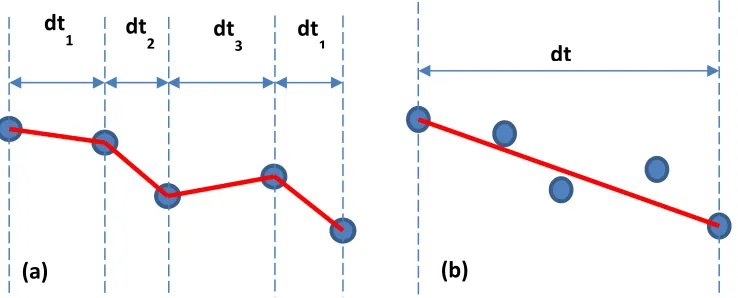
Several methods of integrating the decay data can also be considered. Firstly the previous points may be used individually to calculate multiple B* values which can then be averaged. Sec-ondly a data point several points before, but ignoring those in between, may be used to calculate B*. And finally a trend may be drawn from multiple B* values. For the first and third methods the B* value is calculated using multiple short time steps, as seen in Figure 1(a) whilst the second method uses a larger time step encompassing multiple data points to calculate B* as seen in Fig-ure 1(b).
All three methods were considered for each B*, however after some initial analysis it was found that the most viable was the second method as it produced the most accurate results, there-fore it was studied further and presented herein.
Number of decay data points required
In order to study the number of decay data points required to produce accurate orbit lifetime predictions, historical data of the test case GOCE will be used. At each data point new predictions will be made first using two previous data points to determine the various B* values and therefore the lifetime predictions associated with each. Then three previous data points will be used, and then four and so on until all previous points are used. This method will produce a matrix of orbit
dt
1
dt
3
dt
2
dt
1
[image:3.612.120.489.378.527.2]dt
Figure 1. Decay Data Integration Method Comparison
lifetime predictions which, when compared to the historical data, will produce a matrix of predic-tion errors. This error matrix can then be studied to determine the number of previous data points required to produce the most reliable predictions.
METHOD COMPARISON
In order to compare the accuracy of the various B* formulations the matrix of prediction errors was built by comparing the predictions made to the historical data taken from GOCE’s TLE.18 The input parameters for GOCE considered were the published estimates: mass approximately 1050kg, area approximately 1m2 and the standard assumption of a 2.2 drag coefficient.16
[image:4.612.120.495.305.487.2]As discussed in the previous section all possible numbers of previous data points (N) were considered however due to the abundance of data it cannot be displayed herein therefore a selec-tion is presented for study. Table 1 shows the mean percentage error for each B* with the selec-tion of numbers of previous data points used. To determine this mean percentage error, the per-centage errors in predictions made at each data point are calculated by comparing the predictions to the real lifetimes taken from the TLE, then averaging all of these errors to produce a mean. The standard deviation of the errors is also considered and presented in Table 2.
Table 1. Mean Percentage Error Comparison of Various Methods
N 𝐵
∗ 𝐵
1∗ 𝐵2∗ 𝐵3∗ 𝐵4∗ 𝐵5∗
Error (%) Error (%) Error (%) Error (%) Error (%) Error (%)
2 62.34 66.70 66.70 66.70 62.34 62.34
3 14.56 19.27 19.27 19.27 14.56 14.56
5 11.93 21.63 21.63 21.64 11.93 11.93
10 12.54 41.93 41.93 41.94 12.54 12.54
15 12.57 62.91 62.91 62.91 12.57 12.57
20 12.51 85.45 85.45 85.46 12.50 12.51
50 16.99 291.84 291.84 291.90 16.99 16.99
All 68.44 1847.77 1847.77 1848.39 68.45 68.44
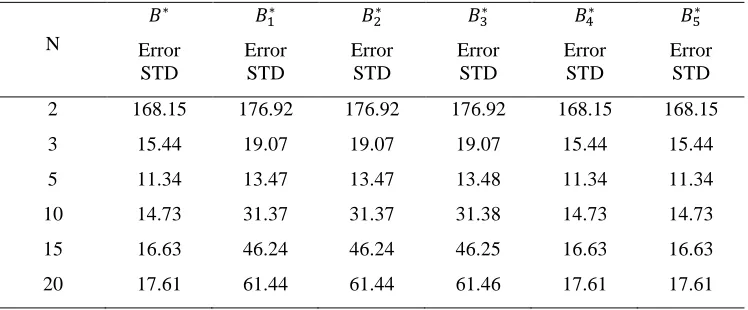
Table 2. Error Standard Deviation Comparison of Various Methods
N
𝐵∗ 𝐵
1∗ 𝐵2∗ 𝐵3∗ 𝐵4∗ 𝐵5∗
Error STD
Error STD
Error STD
Error STD
Error STD
Error STD
2 168.15 176.92 176.92 176.92 168.15 168.15
3 15.44 19.07 19.07 19.07 15.44 15.44
5 11.34 13.47 13.47 13.48 11.34 11.34
10 14.73 31.37 31.37 31.38 14.73 14.73
15 16.63 46.24 46.24 46.25 16.63 16.63
[image:4.612.120.494.522.677.2]50 22.53 163.78 163.78 163.82 22.53 22.53
All 0.79 132.55 132.55 132.60 0.79 0.79
In a cursory examination of Table 1 and 2 similarities are immediately obvious between B*, B4* and B5* and between B1*, B2* and B3*. The chief difference between these two sets is the inclusion or exclusion of atmospheric density in the formulation of B* as is shown by Equations 1-6. The inclusion of density in B* can be seen to have a significantly negative impact on predic-tions accuracy; this effect can also be seen to increase as more and more previous data points are incorporated. This may seem, at first, counter-intuitive, as the general assumption in science is that having more data is always better. However, because the atmospheric density varies greatly with altitude the use of more data points actually introduces a large error into the calculation of B*. It is therefore deemed prudent to exclude atmospheric density from B*.
It can be seen from comparison of B*, B4* and B5* that excluding the density increases the ac-curacy significantly. It can also be seen that the inclusion or exclusion of the mass and atmos-pheric rotation retarding force make very little impact on accuracy. This was to be expected as these parameters have a much smaller uncertainty than the drag coefficient and area, so much so that they create a negligible difference in this method. However, in order to capture the uncertain-ty, small as it may be, in mass as well as for simpliciuncertain-ty, it is recommended that B* be used.
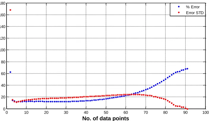
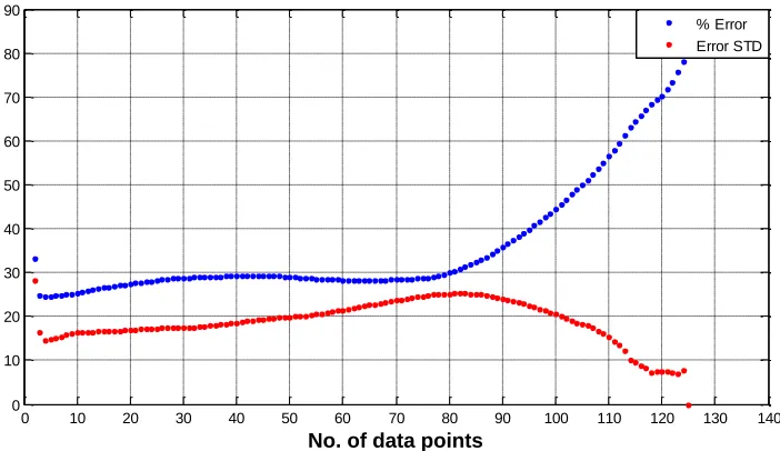
It can also be seen in Table 1 that there appears to be a turning point in the number of previous data points required to produce the best results. In order to better determine what this turning point is, the mean percentage errors for B* were plotted, see Figure 2. This turning point exists due to the variable nature of B*; because the drag coefficient varies depending on atmospheric conditions and the area will also vary as the spacecraft tumbles, B* is not a constant. Therefore as more data points are used the variation in B* is lost in averaging, while using too few data points will fail to capture it accurately.
[image:5.612.135.487.429.633.2]
Figure 2. Accuracy comparison for B* using various numbers of previously data points.
0 10 20 30 40 50 60 70 80 90 100
0 20 40 60 80 100 120 140 160 180
No. of data points
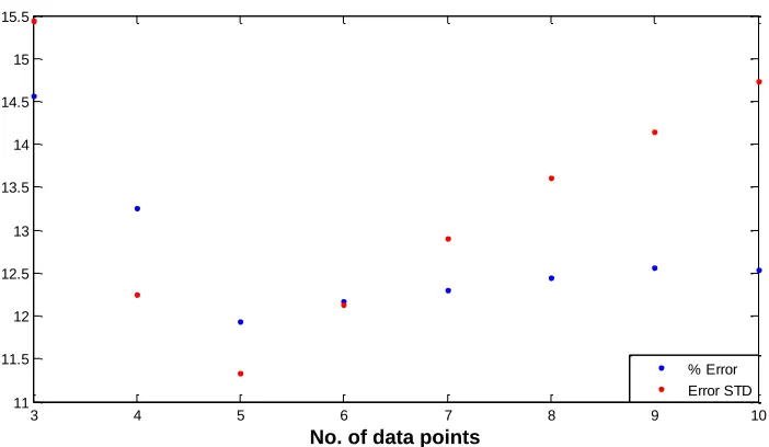
Figure 3. Close Up of Relevant Part of Figure 2.
It can be seen in Figure 2, and more clearly in Figure 3, that the turning point is at using 5 pre-vious data points. Therefore it is recommended that 5 data points be used. A case could be made for using more data as it can be seen that the percentage error remains relatively low between us-ing 3 and 40 points. However when considerus-ing the standard deviation a steady rise can be seen, therefore keeping the number of points used to an absolute maximum of 30 is recommended.
Finally having established the most accurate combination of B*, data integration method and the number of previous data points required, a comparison can be drawn between the original method previously presented by the authors and this updated method. For the same set of data points using the original method and not including any decay data, the mean percentage error was found to be 24.79% (with a standard deviation of 9.61) compared with the 11.93% (standard de-viation 11.34) of the discussed updated method. This demonstrates that the updated method pro-duces a significant improvement in orbit lifetime prediction accuracy. It should be noted here that while the updated method is now immune to errors in the initial input parameters, the previously presented method is highly dependent on them. The assumed input parameters give a B* value of 0.002m2/kg, while the using the decay data to calculate B* gives a mean value of 0.00225 m2/kg from all the predictions. The B* values generated by the new method can be seen in Figure 4.
3 4 5 6 7 8 9 10
11 11.5 12 12.5 13 13.5 14 14.5 15 15.5
No. of data points
Figure 4. Comparison of B* values
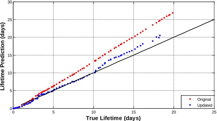
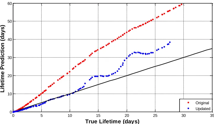
The new method is therefore entirely independent from the original estimates of mass, area and drag coefficient. So taking for example an over estimation of the mass of GOCE to 1100 kg: this produces a mean percentage error in the previous method of 29.39% (standard deviation 9.39) whilst the new method maintains 11.93% error. Predictions at each data point can also be compared, as can be seen in Figure 5.
Figure 5. Comparison of Original and Updated Methods Accuracy
In Figure 5 the solid black line denotes the 100% accuracy or 0% error. As the updated meth-od follows this line much more closely this shows that the updated methmeth-od prmeth-oduces significantly better predictions especially when considering the final 10 days. Within 10 days of re-entry the
20-Oct-130.5 27-Oct-13 03-Nov-13 10-Nov-13 17-Nov-13
1 1.5 2 2.5 3 3.5x 10
-3
Date
B* (
m
2 /kg
)
B* Calculated from Decay Data
B* Calculated from Original Input Parameters Mean of B* from Decay Data
0 5 10 15 20 25
0 5 10 15 20 25 30
True Lifetime (days)
Life
time
Pre
dic
tion (
day
s)
[image:7.612.124.485.392.594.2]updated method produces results that are almost exact, coming within a few hours of the true de-cay time whilst the old method deviates up to approximately 2.5 days.
METHOD VALIDATION
In order to demonstrate that the method presented herein can be applied with success to other spacecraft, several missions were used to demonstrate the success of the method in improving on predictions made by the previous method. All of the missions discussed completed an uncon-trolled re-entry.
GFZ-1
GFZ-1 (COSPAR spacecraft identification 1986-017JE) was a spherical satellite launched in 1995 by GFZ Potsdam to study the Earth’s gravity field. After a successful mission it completed an uncontrolled re-entry in June 1999. The spacecraft initial parameters were: mass approximate-ly 20.63 kg, area approximateapproximate-ly 0.0363m2.19 As with GOCE the final portion of the spacecraft’s re-entry will be studied.
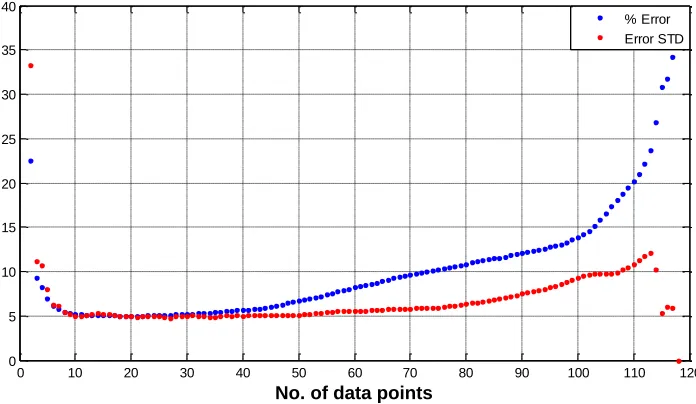
[image:8.612.136.484.362.564.2]Firstly the number of data points used is studied. In this case it becomes clear from Figure 6 that using 5 data points would be less advisable; instead using 10 would be more appropriate. The mean percentage error when using 5 data points was 6.97%, while using 10 points this error drops to 5.23%. This suggests that a greater sample of spacecraft is required to make a better recom-mendation on the number of data points that should be used. It can be seen that as before the per-centage error begins a steady rise and therefore it could be recommended again that no more than 30 previous data points should be used.
Figure 6. Accuracy comparison when using various numbers of previously data points.
The accuracy of the updated and original methods can then be compared, in this case using the 10 previous data points method. It can be seen in Figure 7 that again the updated method is clear-ly more accurate than the original method. The mean percentage error in the original method was 20.63% (standard deviation 10.24) compared to 5.23% (standard deviation 4.98) of the updated method.
0 10 20 30 40 50 60 70 80 90 100 110 120
0 5 10 15 20 25 30 35 40
No. of data points
Figure 7. Comparison of Original and Updated Methods Accuracy
Cosmos 1939
Cosmos 1939 (COSPAR spacecraft identification 1988-032A) was the first operational lite of the Russian/CIS (Commonwealth of Independent States) Resurs-O1 programme. The satel-lite was launched in 1988 to provide geologic applications including fire detection and ice moni-toring. The satellite re-entered at the end of October 2014. The spacecraft initial parameters were: mass approximately 1900 kg, area approximately 11m2. As with GOCE the final portion of the spacecraft’s re-entry will be studied.
Again the number of data points used is studied. In this case it becomes clear from Figure 8 that as with GOCE using 5 data points would be acceptable, however using 10 would also be ap-propriate as with the GFZ-1. The mean percentage error when using 5 data points was 12.98%; using 10 points this error drops slightly to 11.78%. In this case the steady rise in error when using more data points present in the other cases is absent until very late in this spacecraft’s lifetime. However using more data points would bring no material benefit.
0 5 10 15 20 25 30 35
0 5 10 15 20 25 30 35
True Lifetime (days)
Life
time
Pre
dic
tion (
day
s)
Cos
Figure 8. Accuracy comparison when using various numbers of previously data points.
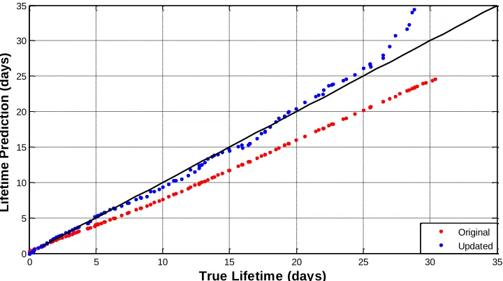
The accuracy of the updated and original methods can then be compared, in this case using the 10 previous data points method. It can be seen in Figure 9 that again the updated method is clear-ly more accurate than the original method. The mean percentage error in the original method was 27.69% (standard deviation 5.53) compared to 11.78% (standard deviation 4.74) of the updated method.
Figure 9. Comparison of Original and Updated Methods Accuracy
0 10 20 30 40 50 60 70 80 90
0 50 100 150 200 250
No. of data points
% Error Error STD
0 5 10 15 20 25 30 35 40
0 5 10 15 20 25 30 35 40 45
True Lifetime (days)
Life
time
Pre
dic
tion (
day
s)
[image:10.612.125.485.410.609.2]UARS
UARS (Upper Atmosphere Research Satellite, COSPAR spacecraft identification 1991-063B) was a NASA Earth observation satellite which was officially decommissioned on December 14th 2005, finally re-entering at the end of June 2011. The spacecraft initial parameters were: mass approximately 5668 kg, area approximately 16.6m2.20,21 Again only the final portion of the space-craft’s re-entry will be studied.
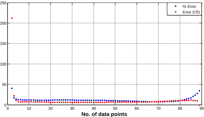
[image:11.612.135.486.236.439.2]As before the number of data points used is studied. In this case it becomes clear from Figure 10 that, as with GOCE, using 5 data points would be advisable. However using 10 points would also be appropriate as with the GFZ-1. The mean percentage error when using 5 data points was 24.59%, while using 10 points this error increases slightly to 25.35%. In this case the steady rise in error when using more data points is present, therefore again it is recommended that no more than 30 data points be used.
Figure 10. Accuracy comparison when using various numbers of previously data points.
The accuracy of the updated and original methods can then be compared, in this case using the 10 previous data points method. It can be seen in Figure 11 that again the updated method is clearly more accurate than the original method. The mean percentage error in the original method was 95.40% (standard deviation 35.98) compared to 25.35% (standard deviation 16.35) of the updated method.
0 10 20 30 40 50 60 70 80 90 100 110 120 130 140
0 10 20 30 40 50 60 70 80 90
No. of data points
Figure 11. Comparison of Original and Updated Methods Accuracy
CONCLUSION
Increased accuracy is achieved by using spacecraft decay tracking data to inform the input pa-rameters used in orbit lifetime predictions. The method presented herein is not affected by errors in the input parameters, as it derives these from the spacecraft decay tracking data. On analysis of the four presented case studies it can be concluded that though in some cases using fewer data points from the spacecraft decay data is slightly more accurate, on the whole using 10 data points is recommended as in all of the presented case studies this leads to reliable predictions. However more case studies should be used to confirm this recommendation.
ACKNOWLEDGMENTS
Emma Kerr would like to give her sincere thanks to the Education Office of the European Space Agency for their support in attending this conference.
REFERENCES 1
Cook, G. E., King-Hele, D. G., and Walker, D. M. C., “The Contraction of Satellite Orbits under the influence of Air Drag I. With Sphericallly Symmetical Atmosphere,”
Proceedings of the Royal Society A: Mathematical, Physical and Engineering Sciences,
vol. 257, 1960, pp. 224–249. 2
Cook, G. E., King-Hele, D. G., and Walker, D. M. C., “The Contraction of Satellite Orbits Under the Influence of Air Drag II. With Oblate Atmosphere,” Proceedings of the Royal
Society A: Mathematical, Physical and Engineering Sciences, vol. 264, 1961, pp. 88–121.
3
King-Hele, D. G., “The Contraction of Satellite Orbits Under the Influence of Air Drag III. High-Eccentricity Orbits,” Proceedings of the Royal Society A: Mathematical,
Physical and Engineering Sciences, vol. 267, 1962, pp. 541–557.
4
Cook, G. E., and King-Hele, D. G., “The Contraction of Satellite Orbits Under the Influence of Air Drag IV. With scale height dependant on altitude,” Proceedings of the
0 5 10 15 20 25 30 35
0 10 20 30 40 50 60
True Lifetime (days)
Life
time
Pre
dic
tion (
day
s)
Royal Society A: Mathematical, Physical and Engineering Sciences, vol. 275, 1963, pp. 357–390.
5
Cook, G. E., and King-Hele, D. G., “The Contraction of Satellite Orbits under the Influence of Air Drag V. with Day-To-Night Variation in Air Density,” Philosophical Transactions of the Royal Society of London A: Mathematical, Physical and Engineering
Sciences, vol. 259, Dec. 1965, pp. 33–67.
6
Cook, G. E., and King-Hele, D. G., “The Contraction of Satellite Orbits Under the Influence of Air Drag VI. Near-Circular Orbits with Day-to-Night Variation in Air Density,” Proceedings of the Royal Society A: Mathematical, Physical and Engineering
Sciences, vol. 303, 1968, pp. 17–35.
7
King-Hele, D. G., and Walker, D. M. C., “The Contraction of Satellite Orbits under the Influence of Air Drag VII. Orbits of high eccentricity, with scale height dependent on altitude,” Proceedings of the Royal Society A: Mathematical, Physical and Engineering
Sciences, vol. 411, 1987, pp. 1–17.
8
King-Hele, D. G., and Walker, D. M. C., “The Contraction of Satellite Orbits Under the Influence of Air Drag VIII. Orbital lifetime in an oblate atmosphere, when perigee distance is perturbed by odd zonal harmonics in the geopotential,” Proceedings of the
Royal Society A: Mathematical, Physical and Engineering Sciences, vol. 414, 1987, pp.
271–295.
9 Sharma, R. K., “Contraction of satellite orbits using KS elements in an oblate diurnally varying atmosphere,” Proceedings of the Royal Society A: Mathematical, Physical and
Engineering Sciences, vol. 453, Nov. 1997, pp. 2353–2368.
10 Sharma, R. K., “Contraction of high eccentricity satellite orbits using K-S elements with air drag,” Proceedings of the Royal Society A: Mathematical, Physical and Engineering
Sciences, vol. 454, 1998, pp. 1681–1689.
11 Sharma, R. K., “Analytical approach using KS elements to near-Earth orbit predictions including drag,” Proceedings of the Royal Society A: Mathematical, Physical and
Engineering Sciences, vol. 433, 1991, pp. 121–130.
12 Sharma, R. K., “A third-order theory for the effect of drag on Earth satellite orbits,”
Proceedings of the Royal Society A: Mathematical, Physical and Engineering Sciences,
vol. 438, 1992, pp. 467–475.
13 Kerr, E., and Macdonald, M., “A General Perturbations Method For Spacecraft Lifetime Analysis,” 25th AAS/AIAA Space Flight Mechanics Meeting, Wiliamsburg, VA, USA: 2015, pp. 1–15.
14 Kerr, E., and Macdonald, M., “A General Perturbations Method for Spacecraft Lifetime Analysis Incorporating Solar Activity,” Under Review for Proceedings of the Royal
Society Open Science.
15 Kerr, E., and Macdonald, M., “Improving the Accuracy of Orbit Lifetime Analysis Using Enhanced General Perturbations Methods,” 66th International Astronautical Congress, Jerusalem, Isreal: 2015, pp. 1–6.
16
International Organisation for Standardisation, 27852:2010(E): Space systems —
Estimation of orbit lifetime, 2010.
17
Drinkwater, M. R., Haagmans, R., Muzi, D., Popescu, A., Floberghagen, R., Kern, M., and Fehringer, M., “The GOCE Gravity Mission: ESA’s First Core Earth Explorer,”
Proceedings of the 3rd International GOCE User Workshop, Frascati, Italy: 2007.
19
König, R., Schwintzer, P., Bode, A., and Reigber, C., “GFZ-1: A small laser satellite mission for gravity field model improvement,” Geophysical Research Letters, vol. 23, Nov. 1996, pp. 3143–3146.
20 Pardini, C., and Anselmo, L., “Reentry Predictions of Three Massive Uncontrolled Spacecraft,” Proceedings of the 23rd International Symposium of Space Flight Dynamics, Pasadena, CA, USA: 2012.
21 Reber, C. A., “The upper atmosphere research satellite (UARS),”
Geophysical Research