Experimental investigation on the effects of surface roughness on microscale liquid flow

Rochester Institute of Technology

RIT Scholar Works

Theses Thesis/Dissertation Collections

2008

Experimental investigation on the effects of surface

roughness on microscale liquid flow

Tim Brackbill

Follow this and additional works at:http://scholarworks.rit.edu/theses

This Thesis is brought to you for free and open access by the Thesis/Dissertation Collections at RIT Scholar Works. It has been accepted for inclusion in Theses by an authorized administrator of RIT Scholar Works. For more information, please [email protected].

Recommended Citation

Experimental investigation on the effects of surface 

roughness on microscale liquid flow

by

Timothy Brackbill

A thesis submitted in

partial fulfillment of the 

requirement for the 

B.S./M.S.

in

Mechanical Engineering

Dr. Satish G. Kandlikar

Thesis Advisor

Department of Mechanical Engineering

Dr. Steven Weinstein

Department of Mechanical Engineering

Dr. Jeffery Kozak

Department of Mechanical Engineering

Dr. Edward Hensel

Department of Mechanical Engineering

Department of Mechanical Engineering

Rochester Institute of Technology

I. Abstract

Microfluidics has become of interest recently with shrinking device sizes.

Roughness structures left from machining processes on the inside of

tubes and channels that were once not a concern may now create relative

roughness that exceeds 5%. Confusion still exists in the literature as to

the extent of the effects of roughness on laminar flow. This work aims to

experimentally examine the effects of different roughness structures on

internal flows in high aspect ratio rectangular microchannels. A total of

four test sections were fabricated to test samples with different patterned

rough surfaces, and to also vary the two opposite surfaces forming the

long faces of the channel. These test sections allowed the same

roughness samples to be tested at varying relative roughnesses and

allowed a systematic study on their effects on pressure drop. The first

test section looked at sawtooth effects on laminar flow. The second

looked at uniform roughness on laminar flow. The third looked at

sawtooth roughness in turbulent flow, and the fourth looked at varying

pitch sawtooth roughness in laminar flow. Rough surfaces were formed in

one of two ways. The first involved making structured repeating sawtooth

ridges with a ball end mill on a CNC machine. The second was using

sandpaper in a crosshatch pattern to make a more unpatterned

roughened surface. In this study, the Reynolds number was varied from

experimental uncertainty in the experimental data is at worst 7.58% for

friction factor and 2.67% for Reynolds number. Roughness structures

varied from a lapped smooth surface with 0.2 μm roughness height to sawtooth ridges of height 117 μm. Hydraulic diameters from 198 μm to 2,349 μm were tested. The highest relative roughness tested was 24.8%.

As a result of the first and second experiments, it was shown that using

constricted parameters, sawtooth and uniform roughness performance

could be predicted in the laminar regime. In the third experiment, it was

shown that certain sawtooth roughness samples cause the results to

converge to a single line for friction factor. In the fourth experiment, the

pitch of sawtooth elements was shown to be a key parameter in showing

when each parameter is applicable. It was found that roughness has an

effect even at relative roughness values less than 5%. Lapped smooth

samples showed no departure from macroscale theory at all channel

diameters tested, which implies that no departure from continuum

mechanics occurred at the length scales tested. This fit with what was

expected. Early transitions to turbulence were seen however, showing

decreasing transition Reynolds number with increasing relative

roughness. The lowest turbulent transition occurred at a Reynolds

number of 210, with a relative roughness of 24.8%. Most all of the

roughness structures studied were found to have experimental results

that were well predicted with the use of constricted parameters.

seen to have experimental results approaching theory calculated with

II.Table of Contents

I. Abstract...2

II. Table of Contents...5

III. Index of Tables and Figures...7

i. Figures...7

ii. Tables...8

IV. Nomenclature...9

1 Introduction...10

1.1 Previous Experimental Studies...10

1.1.1 Laminar and transition studies...10

1.1.2 Turbulent Flow...21

1.2 Numerical/Theoretical Work...23

1.3 Roughness Characterization...27

2 Theoretical Work...30

2.1 Current Roughness and Nikuradse...30

2.2 Derivation of Constricted Parameters...33

2.3 Application of Lubrication Theory...37

3 Experimental Work...44

3.1 Summary of experimental work...44

3.2 Initial Experimental Work – Sawtooth High...46

3.2.1 Experimental Loop Description for initial work...46

3.2.2 Experimental Schematics and Drawings...47

3.2.3 Samples used in First Experimentation...49

3.2.4 Experimental Procedure for the First setup...52

3.3 Second Setup – Low uniform RR testing...52

3.3.1 Experimental Setup for Low RR uniform elements...53

3.3.2 Samples used for low uniform roughness...55

3.4 Third Experiment – Fully Turbulent Flow...57

3.4.1 Experimental Schematics...57

3.4.2 Samples...58

3.4.3 Experimental Procedure...58

3.5 Fourth Experiment – Differing pitches of sawtooth roughness...59

3.5.1 Experimental Schematics...59

3.5.2 Samples...59

3.5.3 Experimental Procedure...62

3.6 LabVIEW...62

3.7 Experimental Uncertainties...67

4 Results...71

4.1 Summary and Major Findings...71

4.2 Results of first Experimentation...72

4.3 Results of second Experimentation...76

4.3.1 Experimental Results...76

4.3.2 Results of applying lubrication theory...78

4.4 Results of Third Experiment – Turbulent experiments...82

4.5 Results of fourth experimentation – varying pitch...84

4.6 Transition to turbulence...86

5 Conclusions...90

6 References...92

7 Appendices...96

7.1 Appendix A – First setup drawings...96

7.2 Second Experimental Setup...109

III.Index of Tables and Figures

i. Figures

Figure 1.1: Modified Moody Diagram by Kandlikar [28]...25

Figure 1.2: Pressure drop v. pitch of sawtooth obstructions for Re = 40, h = 0.1, from Rawool [30]...26

Figure 1.3: Generic roughness surface with parameters marked...29

Figure 2.1: Illustration of Idealized roughness surface from Nikuradse [2]...32

Figure 2.2: Generic ribbed roughness with parameters illustrated...35

Figure 2.3: Illustration of Lubrication Problem...38

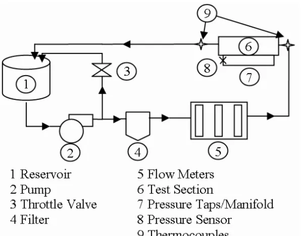
Figure 3.1: Schematic of the first test loop designed...49

Figure 3.2: Left: Exploded view of the setup Right: Assembled setup without cover piece...49

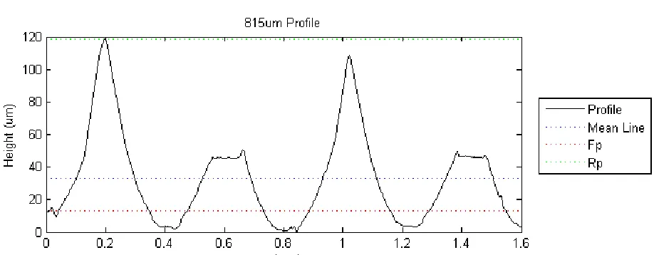
Figure 3.3: 405um pitch profile, taken with a stylus profilometer. The parameters are marked...51

Figure 3.4: 815um pitch profile, taken with stylus profilometer...51

Figure 3.5: Ground smooth sample surface, taken with a stylus Profilometer...52

Figure 3.6: Isometric Schematics of New Test section...54

Figure 3.7: Schematic of test loop used for low Relative roughness testing...56

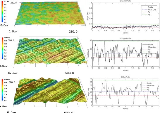
Figure 3.8: 3D microscope images and stylus profilometer scans of the three roughnesses tested...58

Figure 3.9: Test loop for third experimentation...59

Figure 3.10: 3D Microscope compilations and 2D stylus profilometer scans of the samples...60

Figure 3.11: Interferometer scans (left) and apparent 2D profile scans (right) for the three samples tested...63

Figure 4.1: Smooth channel verification with Dh = 565um...74

Figure 4.2: Uncorrected - aligned sawtooth roughness p=405μm, Dh=1240μm, b = 653μm...75

Figure 4.3: Corrected - aligned sawtooth p=405μm, Dhcf=847μm...76

Figure 4.4: Comparison of the two different pitches with the same constricted hydraulic diameter...76

Figure 4.5: Representative samples from the low uniform roughness testing plotted with (a) root parameters (b) constricted parameters...78

Figure 4.6: Illustration of all parameters used in experimentation applied to the

60 grit channel profile...79

Figure 4.7: Variation of beff,exp with Reynolds Number...80

Figure 4.8: Parameters for separation normalized with experimental results...81

Figure 4.9: Results of turbulent testing with 405um samples (a) a single test plotted with a prediction of friction factor (b) all the samples...83

Figure 4.10: Comparing the two different sawtooth pitches...85

Figure 4.11: Constricted friction factor vs Reynolds number for 3 varying pitches ...86

Figure 4.12: Constricted friction factor vs Reynolds number for the largest pitch, plotted with both root and constricted parameters...87

Figure 4.13: f*Re vs Beta for the samples with varying pitch...88

Figure 4.14: Transition Reynolds number vs Relative Roughness...90

ii.Tables

Table 3.1: Summary of Roughness in First Experimentation...50

Table 3.2: Description of roughness surfaces used in low RR testing...57

Table 3.3: Summary of machining for the fourth set of samples...61

Table 3.4: State points to reference density...66

Table 3.5: Summary of max errors used in uncertainty analysis for the pressure and flow sensors...71

Table 4.1: Summary of all experimental work. Each row represents an individual test...72

Table 4.2: Repeatability...73

Table 4.3: Summary of experimental results from lubrication theory...80

IV.Nomenclature

α = aspect ratio

αcf = constricted aspect ratio

A = cross sectional area of channel

Acf = constricted cross sectional area of channel

a = channel base

b = channel height

bcf = constricted channel height

beff = separation from lubrication theory

accounting for roughness effects

beff,exp = effective separation from experiments

beff,theory = effective separation from theory

ε = roughness element height

εFP = roughness height - new parameters

δ = used to show uncertainty in trailing variable

Dh = hydraulic diameter

Dh,cf = constricted hydraulic diameter

Dt = root diameter of circular tube

f = friction factor

fMoody = turbulent friction factor from Moody

diagram

Fp = floor profile line

G = mass flow rate

g = gravity vector

h = height of silicon channels

L = a length along the channel in the flow

direction

˙

m = mass flow rate

n = number of points in a roughness profile

sample

p = pitch of roughness elements

P = perimeter or pressure in derivations

Pcf = constricted perimeter

ρ = density of the water

Ra = average roughness

Re = Reynolds number

Rec = critical Reynolds number

Recf or Recf = Reynolds number, calculated from

Dh,cf

Q = volumetric flow rate

Reo = Smooth channel turbulent transition

Rp = maximum peak height

RSm = mean spacing of irregularities

Tmean = mean fluid temperature in test section

ux = fluid velocity component in the x direction

uy = fluid velocity component in the y direction

uz = fluid velocity component in the z direction

V = flow velocity

˙

V = Volumetric flow rate

w = width of silicon channels

x = distance from channel beginning

Z = height at any given point along a roughness

profile (μm)

1 Introduction

Work in the area of roughness effects on friction factors in internal flows

was pioneered by Colebrook [1], Nikuradse [2], and Moody. Their work

was limited to relative roughness values of less than 5%, a value which

may be exceeded in microfluidics application where smaller hydraulic

diameters are encountered. Many previous works have been performed

through the 1990s with inconclusive and often contradictory results. No

studies have been performed that systematically varied the roughness

structures and relative roughness while collecting enough data necessary

for any valid conclusions to be drawn. This study aims to conduct

systematic experiments to evaluate the effects of these roughness

elements on flow.

1.1 Previous Experimental Studies

1.1.1 Laminar and transition studies

Wu and Little [3] noticed an early transition to turbulent flow in

microminiature refrigerators. Their channels were etched on glass and

silicon with Dh from 45.46 to 83.07μm. Wu and Little [4] fabricated

microchannels with the same process, but varied Dh from 134μm to

164μm, and found unusually high frictional factors. They found these to

contribute to low critical Reynolds numbers from ~400-900.

Peng et al. [5] machined five different microchannels in stainless steel,

with Dh ranging from 133μm to 343μm and aspect ratio varying from

0.333 to 1. The error was ±10% on friction calculations and ±8% on

Reynolds number. The fluid used was water, with Reynolds numbers

varying from 50 to 4000. Critical Reynolds numbers were found to be

between 200 and 700, or much lower than conventional macroscale

theory. In this study, Peng stresses the effect of the aspect ratio and

hydraulic diameter on ReC and f. He found that the lowest friction factor,

lower than macroscale theory, occurs at aspect ratios nearest to 0.5. The

ReC value was related to Dh, but no relationship was given. Also noted is a

deviation from classical theory and suggestion that different laminar and

turbulent flow mechanisms are occurring, along with a decrease in the

transition region with decreasing Dh. As such, an empirical relationship

for friction factor is proposed in equation 1.1, where Cf and Cf,t are

empirical constants that are depended on channel aspect ratio and fluid

species.

f_laminar= Cf

Re1.98

f_turbulent= Cf ,t

Re1.72

(1.1)

Pfund et al. [6] used a variable depth microchannel along with pressure

drop sensors and flow visualization to study the same phenomena.

Overall the setup is similar in nature to the setup in use for this thesis.

The samples used to construct the channel were characterized with an

optical profilometer, however for the rough channel only one side of the

rectangular channel’s 128 μm – 1,050 μm by 10 mm dimensions were

roughened. Uncertainties as found with a Monte-Carlo simulation were

stated to be between ±5.4% and ±11.1%, although it is stated that RMS

calculations yield 1% higher uncertainties. Uncertainties in Reynolds

number were between ±1.6% and ±3.4%. It was found that every

channel used in the study exhibited higher than theoretical predictions in

the laminar region, even for the smooth channels. For the roughened

channels, the discrepancy was even more pronounced. ReC was again

observed to be lower than theory, but not as extreme as those reported

by Peng et al. [5]. Again, a dependence of Rec on hydraulic diameter was

observed. Utilizing flow visualization, eddy currents around surface

features are proposed to be the mechanism for transition, and also for the

shorter but continuous transitions reported elsewhere.

Tu et al. [7] performed tests on five microchannels with hydraulic

diameters from 69.5 μm to 304.7 μm and aspect ratio from 0.09 to 0.24.

Working fluid was R134a liquid or vapor depending on the test. The test

sections were manufactured such that the surfaces were as smooth as

possible. Errors were reported as ±6.3% max for f and ±2% max for Re.

It was found that for the four channels with relative roughness less than

0.3%, no deviation occurred from conventional f or ReC macroscale theory

(ReC 2150 to 2290 was reported). For the one channel with a relative

roughness of 0.35%, the friction factor was observed to be 9% higher than

predicted, accompanied by a significantly lower ReC of 1570.

Wu et al. [8] used thirteen fabricated trapezoidal silicon channels with

pairs of geometrically similar channels with varying surface roughness

and hydrophobicity (through use of SiO2). An increased friction factor was

observed in the laminar flow regime due to surface roughness when

compared to the smooth channel. Increasing discrepancies were noted

with increasing Re for the smooth versus roughened channels. The

coating of SiO2 also slightly increased friction factor values from the

smooth channel. The oxide also increased the convective heat transfer.

Wu also describes empirical correlations for Nu and fappRe for the

geometric ratios relating to trapezoidal channels.

Celata et al. [9] used capillary glass tubes with hydraulic diameter ranging

from 70 μm to 326 μm with water as the working fluid. The inside of the

capillaries were roughened by flowing particulates through the channels.

It was observed that even the low relative roughness values seemed to

increase friction factor in the laminar region in comparison to the smooth

channel results. Additionally, earlier transitions were seen with the

roughened channels.

Mala et al. [10] conducted a study on 13 capillary tubes with hydraulic

diameter ranging from 50μm to 254μm. This study has a reported

roughness height values of 1.75μm. These channels are considered

smooth in this study, which is interesting when it is noticed these are

rougher than the “rough” capillaries used by Celata et al. [9]. Mala

explains the discrepancy with a modified roughness-viscosity theory. This

model varies the viscosity of the fluid going around the roughness

elements and increases the pressure drop prediction. This modified

model is based on an older aerodynamic model by Merkle et al. [11] and

Tani [12]. The model relies on the results of CFD experimentation, and is

not applicable to any surface.

Kandlikar et al. [13] studied heat transfer and pressure drop in stainless

steel capillary tubing of diameters 620μm and 1067μm. Three different

surface types for each diameter were created using varying acid etching

techniques on the inside of the capillaries. For the larger diameter, little

effect on friction factor or heat transfer performance was discernible from

even the largest relative roughness value of 0.23%. It was suggested that

this diameter is not truly microscale, and thus macroscale theories are

more applicable. For the smaller diameter, the highest relative roughness

value of 0.36% yielded the highest friction factors and highest heat

transfer performance. The capillaries with successively smoother walls

showed less extreme friction factor and heat transfer.

Baviere et al. [14] studied both the effect of roughness and the effect of

the electrical double layer on internal flows. The study used silicon

etched channels for hydraulic diameters less than 100μm and a bronze

block setup for hydraulic diameters greater than 100μm. Roughness elements were created by embedding SiC particles in a thin nickel wall

coating. They found no deviation from conventional theory for smooth

channels. In roughened channels, higher friction factors were observed.

However, in contrast to other studies, the addition of roughness elements

in this setup stabilized flow, and created higher values for the transition to

turbulence.

Hao et al. [15] performed an experimental study with etched silicon

rectangular microchannels which had three artificially created roughness

elements on one side of the channel, measuring 50μm square and spaced

between 7 and 8 mm from each other. Hydraulic diameters ranged from

153μm -191μm, and Reynolds numbers were tested with values less than

2400. Flow visualization was also included to observe the flow as it

traversed the artificially created roughness. Smooth channels were

observed to follow conventional theory for friction and transition. The

artificially roughened channels, however, followed conventional theory to

Re = 900, then departed into transition. This study showed that these

elements are able to trigger early transition from laminar by imparting

additional disturbances to the flow. The friction factor remained constant,

which can be explained by the few and sparsely spaced roughness

elements. These did not have a significant effect on the friction factor.

Finally, Hao also concludes that similar features of macroscale turbulence

are also visible in microscale fluid turbulence.

Weilin et al. [16] fabricated trapezoidal channels using micromachining

techniques on silicon substrates. Due to the silicon’s surface finish,

relative roughness values varied from 2.4% to 3.5%. Experimentation

was limited to a 1,723 kPa maximum pressure drop, beyond the silicon

substrate failed. The resulting Reynolds numbers were less than 1500.

They found friction factors that were higher than theory would predict,

and also found linear relationships between pressure drop over length and

Reynolds number to possess higher than theoretical slopes. Using this

data, they applied the modified roughness-viscosity model of Mala and Li

[10] and obtained good correlation with experimental data. A

complicated formulation for a coefficient inherent to the model is

determined using variables such as channel geometry, roughness

distribution, and shape of roughness elements. The coefficients obtained

have limited applicability past the channels used in this study.

Shen et al. [17] machined 26 parallel microchannels of 300μm width and

800μm depth in a copper block. They studied the effects of 4% relative

roughness on friction factor and Nusselt number. No effect on the

transition to turbulence was found, however Reynolds numbers were

tested only to 1257, which severely restricts any conclusions of this

nature. It was also found that for low Reynolds numbers no departure

from macroscale theory was observed. With increasing Re, the Poiseuille

number increased along with Re rather than remaining constant. They

proposed the correlation given in equation 1.2 for roughened rectangular

microchannels and laminar flow.

f Re0.4743=4.0922 (1.2)

Celata et al. [18] used a parallel microtube setup (Dh=130μm) with steam

condensation heating to study the effects of roughness on heat transfer

and fluid flow. It was found that below Re = 583 the roughness did not

play a major role, and friction factor agreed with macroscale theory. The

critical Reynolds number was found to range from 1881-2479 for laminar

to turbulent transition. They also observed poor fit of experimental heat

transfer performance with established correlations.

Li et al. [19] used a variety of stainless steel, glass, and fused silica

capillary tubes to study the effects of roughened tubes. Hydraulic

diameters ranged from 79.9-449μm. The fused silica and glass tubes

were considered to be smooth tubes for this experimentation, as the

roughness was negligible. The stainless steel tubes had relative

roughness ranging from 3-4%. No deviation from macroscale theory was

found in the smooth microtubes. For the rough stainless steel tubes, f*Re

was found to be much higher. As the relative roughness increased, larger

discrepancies were opserved. The parameter f*Re was again shown to

vary with Reynolds number in this work instead of remaining constantas

macroscale theory would predict.

Bucci et al. [20] tested stainless steel capillaries with hydraulic

diameters from 172μm to 520μm. The study used vapor condensation

heating for the heating source. It was shown that for low relative

roughness, the tubes behaved as macroscale theory predicts, with both

experimental friction factor and laminar-turbulent transition agreement.

For rougher tubes with smaller diameters, the laminar-turbulent transition

was observed at higher Reynolds numbers and very abrupt rather than

smooth.

Schmitt and Kandlikar [21] performed work in this area using

rectangular minichannels of hydraulic diameters ranging from 325μm to

1819μm with air and water as the working fluids. They found early

turbulent transition and higher pressure drops when compared to

conventional values. They also found that the laminar friction factor could

be calculated by using the constricted hydraulic diameter, Dh,cf. Use of

this constricted area takes into account only the area of the channel that

has no roughened protrusions into the flow. They also found a

relationship between the critical Reynolds number and the relative

roughness.

Wibel et al. [22] performed experimentation on varying aspect ratio

microchannels, fabricated with an end mill in metal. The hydraulic

diameters were intended to be a constant 133μm, but manufacturing

inaccuracies led to minor variations. Three aspect ratios were

investigated, unity, 1:2 and 1:5. An increasing critical Reynolds number

was found with decreasing aspect ratio, with Rec=1800-2000 for a unity

aspect ratio and Rec=2300-2800 for 1:5. It was also found that

decreasing aspect ratio increased the length of the laminar turbulent

transition. Good correlation was found with conventional macroscale

theory for friction factors, however the channels were relatively smooth.

Campbell et al. [23] showed that the type of entrance to the mini- or

micro-channel has little effect on pressure drop or laminar turbulent

transition. This result verifies that the above studies can indeed be

compared as they all implement differing test setups and entry

conditions.

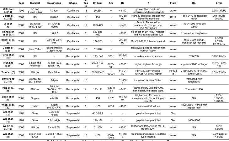
A summary of experimental works is presented in Table 1.1.

Year Material Roughness Shape # Tes

ts

Dh (μm) h/w Re f Fluid Rec Error

Mala and Li [10] 1999

SS and

Fused Silica 1.75μm Capillaries 13 50-254 ~ <2100

greater than predicted,

increases w/ decreasing Dh Water 9.2%f 3%Re

Celata et

al. [18] 2000 SS 0.0265 Capillaries 1 130 ~

100-80 00

Re<583 classical, greater with higher Re numbers R114

1881-2479 is transition region

9%f 5%Re 20%Nu

Li et al.

[19] 2000

SS, fused silica, glass

0.1%RR to

4%RR Capillaries 12 79.9-449 ~ <2400

Smooth Tubes follow macroscale, Rough have

15-37% higher f

Water 1700~1900 for rough _tubes

Kandlikar

et al. [13] 2001 SS 1.0-3.0 Capillaries 6

620 and

1067 ~ <2300

no effect on Dh 1067, highest f

and Nu from roughest 620 Water Lowered w/ roughness

Bucci et al.

[20] 2003 SS

0.3% to 0.8%

RR Capillaries 3 172-520 ~

200-60

00 Re<800-1000 follows classical Water

1800-3000, abrupt transition for high RR

8.36%f 1.8%Re 22.25%Nu

Celata et

al. [9] 2004 glass, Teflon

.05μm smooth,

.2-.8μm rough Capillaries 10 31-326 ~

tentatively propose higher than normal friction Water

Peng et al.

[5] 1994 SS ~ Rectangular 7 .133-.343 .333-1

50-400

0 α makes some +, some - Water 200-700 10%f, 8%Re

Pfund et al. [6] 2000

Lexan and Polyimide

.16 and .09μ,

rough 1.9μ Rectangular 6

252.8-190 0

. 0128-.

105

<3600 higher, highest for rough Water approach 2800 w/ larger 11.1%f 3.4% _Red

Tu et al. [7] 2003 Silicon Ra < 20nm Rectangular 5 69.5-304.7 _09-.24. 112-91_{80 RR=.35% f is 9% higher}RR<.3%, conventional, RF134_a 2150-2290 w/ RR<.3%, _{1570 for .35%} 6.3%f 2%Re

Baviere et al. [14] 2004

Bronze, Ni,

SiC, Silicon 5-7μm Rectangular 10

. 01-800

0

increased laminar friction Water increased with _roughness

Hao et al.

[15] 2006 Silicon

Artificial 50x50μm RR

19%

Rectangular 4 153-191 0.39-0_.55 <2400 _{then higher, indicating trans.}follows theory until Re=900, Water Transition ~900

Shen et al.

[17] 2006 Copper 4% RR Rectangular 1 436 0.375

162-12 57

Higher, and Po number increases with Re, nothing at

low Re

Water N/A

7.1%f 6.95%Re 5.93%Nu

Wibel et al.

[22] 2006 metal

1.3μm

(~0.97%RR) Rectangular 6 ~133 0.2-1 <4000 near classical values Water

1800-2300 - varies with aspect ratio

Wu et al.

[3] 1983 Glass

0.05-0.30

height Trapezoidal 45.5-83.1 ~ ~ greater than predicted Gas

Wu et al.

[4] 1984 Glass 0.01 height Trapezoidal 134-164 ~ ~ greater than predicted Gas 1000-3000 Weilin et

al. [16] 2000 Silicon 2.4%-3.5% Trapezoidal 6 51-169 ~ <1500 Higher and larger slope for Px-Re (18-32%) Water N/A 4.6%Re7.6%f

Wu et al.

[8] 2003

Silicon and SiO2

3.26e-5-1.09e-2 Trapezoidal 13 ~100

. 0382-.

3573

14-110 0

roughness increased it, surface

type varied it Water N/A

10.3%fappRe 7.8%Nu

Table 1.1: Summary of Experimental works on the effects of roughness on flow

1.1.2 Turbulent Flow

The effects of roughness in turbulent flow in microchannels is rarely

studied, due to the high pressure drops that this regime requires in small

channels. In addition, most processes of interest in microfluidics work

with laminar flow. Because of this, few studies ever cover this range and

those will be outlined below.

Celata et al. [24] studied the heat transfer on 6 capillary tubes of

diameter 130 μm. The roughness element height in these channels was

3.45 μm, leading to a relative roughness of 2.65%. In the laminar regime,

the experimental results follow closely with theory, however nearly all the

data points collected fall above this line, in agreement with the author's

past work on the laminar regime. In the turbulent regime, the

experimental data fall between the Blasius correlation (smooth tubes) and

Colebrook (for the roughened parameters) predictions. They found that

the Colebrook equation over predicted the results in the turbulent regime.

Bucci et al. [25] used stainless steel capillary tube ranging from 172 μm

to 520 μm with water Reynolds numbers up to 6000. The roughness in

these capillaries varied from 1.49 μm to 2.17 μm. For the largest two

capillary tubes where the turbulent flow regime could be easily reached,

the results matched results that were obtained using the Colebrook

equation.

Tu and Hrnjak [26] tested RF134a in 5 different rectangular channels with

differing aspect ratios. Their relative roughnesses varied from 0.14% to

0.35%. They found excellent agreement with macroscale theory in all

regimes of flow. The turbulent data was found to fit the Colebrook

equation at all roughnesses tested.

Bavier et al. [27] examined friction factor in channels varying from 7 μm to 500 μm. Based on plots presented in the work, it appears that their experimental results in the turbulent region correlate well to macroscale

theory, however it was never explicitly summarized.

Most all previous work on roughness, even in macroscale focuses on

channels with less than 5% relative roughness. Most fluidic devices fall

within this region, however surpassing this limitation is possible and likely

as fluid devices' channel size decreases. Kandlikar et al. [28] proposed

using a constricted parameter, εFP to model roughness in channels. First,

the use of a new roughness element height is proposed by the parameter

εFP. By changing the base dimension of the channel and recalculating

parameters, one can obtain a set of constricted parameters. Using this

method, they proposed a modified Moody diagram to account for the

effect of roughness essentially decreasing the free flow area of a circular

channel. They propose replacing the friction term in the Colebrook

turbulent friction factor equation with the following relation. In this

equation, Dt is the root diameter of the tube

fMoody, cf=fMoody

[

Dt−2FP

Dt

]

5

(1.3) When this is used to replot the Moody diagram, all values of relative

roughness between 3-5% plateau to a friction factor of f=0.042 for high

Reynolds numbers. It is difficult to find a work that tests relative

roughness up to or over 3%, part of this thesis aims to test past this

region.

1.2 Numerical/Theoretical Work

Kandlikar, et al [29] report laminar-to-turbulent transitions at far lower

values than the accepted value of Re=2300. It was shown, citing work by

Schmitt and Kandlikar [21] that increasing relative roughness values

resulted in decreasing critical Reynolds numbers. They give the relation

governing the critical Reynolds number in equation 1.4. Also resulting

from this work is a modified Moody Diagram, based on constricted

hydraulic diameter determining the friction factor. This is shown in Figure

1.1.

0 

D_h,cf0.08 Recrit , cf=2300−18,750





D_{h ,cf}



0.08 

D_{h , cf}0.15 Recrit ,cf=800−3,270





D_{h, cf}−0.08



(1.4)

Figure 1.1: Modified Moody Diagram by Kandlikar [28]

Rawool et al. [30] performed a numerical simulation of sawtooth

roughness elements, similar in nature to those used in this experiment. In

the simulation, serpentine channels were examined. They found that

differing pitches of identical triangular roughness elements led to

variations in pressure drop, and velocity profiles. Pressure drop

decreases with an increase in the pitch of the elements. A diagram of this

discrepancy can be found in Figure 1.2.

Figure 1.2: Pressure drop v. pitch of sawtooth obstructions for Re = 40, h = 0.1, from Rawool [30]

Kandlikar [29] performed a review of available literature and commented

on past and current work in roughness and pressure drop. He concluded

that work much older than the 1990s on microscale pressure drop

included uncertainties that prevented accurate conclusions from being

drawn. It also reaffirmed the effect of surface roughness on friction factor

and early turbulent transition, while calling for more low relative

roughness experimentation.

Chen and Cheng [31] created a fractal and an empirically based model to

determine the pressure drop in roughened microchannels. They

determined a parameter D, that is based on the number of boxes (N) in a

1 Introduction - 1.2 Numerical/Theoretical Work Page 25

uniform square mesh which contains a piece of a superimposed

roughness profile. They systematically decreased the mesh spacing and

plotted the results to obtain an empirical constant. Two additional

empirical constants are then derived from experimental data by Pfund [6].

Bahrami et al. [32] modeled a randomly roughened surface on the walls of

circular microtubes using a Gaussian distribution in both the angular and

longitudinal directions. The total surface shape was represented by a

superposition of these distributions. After solving the NS equations for

this geometry, they arrived at a modification factor that is based on

simply the constantly changing radius. It is then manipulated to an easily

applied form when the roughness height and some additional modification

correlations are given. Using this model Bahrami found agreement with

data published by Celata [18], Jiang [33], Kandlikar [13], Li [19], and Mala

and Li [10]. Although error from the model is never presented in

numerical fashion, average error from the model’s results is about 7%

judging from the 10% error bars used. The error range is from 0-20%.

Zou and Peng [34] used constricted flow parameters with an additional

factor to predict the frictional behavior of flows. To represent the

roughness, they used Rz roughness, or mean peak height. Using just this

constriction in the flow area they described friction factor as a

modification of the standard friction factor, f0. They further modified this

constricted flow parameter by adding empirical correction factors for the

separation between the roughness elements. The separation correction

effectively decreases the original modification factor by adding another

coefficient. Using the height of the roughness elements, the distance

between elements, and the distance to reattachment behind the elements

from backwards facing step results, they then further modified the model.

Mala and Li [10] proposed a roughness viscosity model based on work by

Merkle [11]. The goal of this model is to treat the roughness effects as a

higher apparent viscosity in the fluid near the rough walls. Using this

modified viscosity they rewrote the momentum equation to account for

the roughness effect. The resulting equation is difficult to solve

analytically and as such Mala and Li developed a numerical scheme to

solve it. Using experimental data and CFD results, some empirical

constants are introduced to account for the observed effects.

Some of the models described above account for geometric shape,

however none account for flow effects with anything other than empirical

correction factors. The work presented here is a continuation of our

efforts to develop a model that will account for the fluid flow intricacies,

beginning with lubrication theory.

1.3 Roughness Characterization

Recently, Kandlikar et al. [28] proposed new roughness parameters of

interest to roughness effects in microfluidics. These parameters are

illustrated graphically in Figure 1.3. The parameters are listed below, as

well as how all were calculated. These values are established to correct

for the assumption that different roughness profiles with equal values of

Ra, average roughness, may have different effects on flows with variations

in other profile characteristics. For example, a roughness surface with

twice the pitch but the same Ra may have different pressure drops.

Figure 1.3: Generic roughness surface with parameters marked

• The Mean Line is the arithmetic average of all the points from the raw profile, which physically relate to the height of each point on the surface. It is calculated by equation 1.5. Note that Z is the height of the scan at each point, i.

Mean Line=1

n

∑

n

Z_i (1.5)

● Rp is the maximum peak height from the mean line, which translates to

the highest point in the profile sample minus the mean line. It is calculated by equation 1.6.

Rp=maxZ_i−Mean Line (1.6)

● RSm is defined as the mean separation of profile irregularities, or the

distance along the surface between peaks. This is also defined in this

paper as the pitch of the roughness elements. It can be seen in Figure 1.3.

• Fp is defined as the floor profile. It is the arithmetic average of all the points that fall below the mean line value. As such, it is a good descriptor of the baseline of the roughness profile. It can be calculated from equation 1.7. This value defines the unconstricted parameters.

Let z⊆Z s.t. all z_i=Z_i iff Z_iMean Line

F_p= 1

n_z

∑

n

z_i (1.7)

● FdRa is defined as the distance of the floor profile (Fp) from the mean line.

It is found with equation 1.8.

FdRa=Mean Line−Fp (1.8)

● εFP, or the value of the roughness height, is determined by equation 1.9.

_FP=RpFdRa (1.9)

2 Theoretical Work

2.1 Current Roughness and Nikuradse

A brief look will be taken at the method used by Nikuradse [2] to

generate the original data on roughness in 1933. Nikuradse collected

pressure drop data on roughened pipes, using sand grains as roughness

elements in commercially available smooth tubes. He defined roughness

height to be the diameter of the grains of sand coating the walls of the

pipe. Unfortunately, relating a real life roughness profile to a sand grain

diameter for calculations is nearly impossible. Therefore, a parameter to

relate roughness encountered in microchannels and minichannels to the

data collected by Nikuradse needs to be determined. To begin, the

method Nikuradse used to create his roughness must be examined.

Nikuradse [2] first sifted grains from ordinary building sand to

obtain grains that were 800μm in diameter using an 820μm and a 780μm

sieve. These grains were then put under a micrometer to verify the

desired size. Pipes used in the experiments were filled with a lacquer,

drained, and allowed to become tacky. When the lacquer became tacky,

the pipes were filled with the sieved sand, and then emptied again. He

then again filled the tubes with lacquer and emptied them, in the interest

of achieving better adhesion of sand grains to the walls of the tubes. To

allow the lacquer to properly dry, heat lamps were applied over an

extended amount of time. These pipes were then tested in the

experimental apparatus. The resulting surface of the pipes looks

something like the ideal surface given in Figure 2.1 (b).

Figure 2.1: Illustration of Idealized roughness surface from Nikuradse [2]

A question this process brings to mind is whether a coating of

lacquer over the sand grains would appreciably change their diameter.

To alleviate this worry, Nikuradse applied this same procedure to a flat

plate, and measured the height of the resulting roughness formations

post-lacquering with a micrometer. Confirmation of the height of

roughness was expressed in his work. A microscope picture of these

grains was taken, and it showed that small gaps were present in between

the sand grains, however this illustration was included only to show that

the hydrodynamic influence of these grains was indeed the diameter.

Thus the gap size between the grains is of definite variability from grain to

grain, but from the microscope photo shown in Nikuradse’s work it

appears to be at most 400μm and at least 100μm as a rough estimate.

A model is made, assuming the sand grains are perfect spheres, of

an ideal representation what a 2D stylus profilometer scan of this surface

would look like. This model is implemented in a spreadsheet. Using this

ideal example profile, just as one would use the results of a stylus

profilometer, parameters of the surface can be determined. Since the

average gap distance between grains is not noted in the paper, the

exercise was performed for many gap sizes. With a reasonable

assumption that the average distance between grains is taken to be

300μm; the resulting Ra is 291μm and the proposed parameter εFP is

756μm. The value that Nikuradse would have used for this profile is

800μm, and thus that is what the currently compiled body of data for

friction factor relies on. This alone shows the inadequacy of using the Ra

parameter as roughness height. Both the profile of roughness (at 300μm

gaps between sand grains) and the plot of the parameters versus the gap

size can be seen in Fig. 2. In addition, Figure 2.1 (a) shows clearly that

using εFP the roughness height asymptotically approaches 800μm, which

would be the value that the modern Moody Diagram is based on. Using Ra

as the roughness parameter will give a smaller value of roughness than

intended, and will introduce large errors in the Moody diagram

representation.

Note that with increasing gap size, εFP approaches the actual sand

grain size. One could observe that use of the peak-to-valley roughness

parameter, which is simply the maximum point in the profile subtracted

by the minimum point, would yield the correct size of 800μm. However

practical applications with non-ideal roughness require a parameter that

is easy to calculate with simple algorithms, and peak-to-valley would be

wrong in any case where a profile contained errant peaks or valleys. This

simple exercise shows that εFP can characterize roughness height well on

a theoretical level, wheras the use of Ra is a poor choice.

2.2 Derivation of Constricted Parameters

The derivation of constricted parameters is paramount to determining

important predictors for the friction factor in high roughness channels.

First, we have to define the constricted channel height. An ordinary

channel has a cross section of height b, and width a. However, with

roughness on 2 sides of the channel we will introduce the parameter bcf,

to be the new constricted channel height. These parameters are

illustrated with generic ribbed roughness in Figure 2.2.

Now, to recalculate new constricted parameters, we will use bcf in place of b.

The constricted height, bcf is simply b minus 2εFP. Where area is given by

equation 2.1, constricted area, Acf, will be defined by equation 2.2.

A=ab (2.1)

A_cf=a b_cf (2.2)

Perimeter of the rectangular channels is found using equation 2.3. The

constricted perimeter is found using bcf again instead of b in equation 2.4.

P=2a2b (2.3)

P_cf=2a2b_cf (2.4)

Hydraulic diameter is calculated using equation 2.5. The constricted

hydraulic diameter is found by using the constricted area given in

equation 2.6.

D_h=4A

P (2.5)

D_{h, cf}=4Acf

P_cf (2.6)

Using these constricted parameters, we can now find the theoretical

experimental friction factors. In the laminar regime, friction factor for

rectangular channels is predicted by Kakac, et al [35] by equation 2.7.

2 Theoretical Work - 2.2 Derivation of Constricted Parameters Page 34

The aspect ratio α is defined by equation 2.8. Again, the constricted

aspect ratio, αcf, is defined with the constricted channel height in equation

2.9.

f=24

Re



2

−1.701230.95644−0.25375



=b

a (2.8)

cf=

b_cf

a (2.9)

The theoretical friction factor is calculated using equation 2.10 from

Colebrook [1].

1

f_Moody0.5 =−2.0log



_FP

D_h

3.7 

2.51

Re f0.5_Moody



(2.10)

To relate the turbulent friction factor we have to look at the governing

equation determining friction factor. From the pressure drop equation, we

perform the following derivation for equation 2.11 with channel dimension

based parameters of the terms pulled outside the parentheses.

P=2fmoodyLv

2

D_h

f_Moody=P

x

D_h

2



A



2

f_Moody=P

x

D_hA2

2Q2 f_Moody=



x

1

2Q2



(2.11)

f_{Moody, cf}=



1

2Q2



2

(2.12) To compare the friction factor of the constricted channel, we will

substitute Dh,cf for Dh and Acf for A. Then, equation 2.11 for fMoody will be

divided by equation 2.12 for fMoody,cf to obtain a correlation for the

constricted friction factor. This is given in equation 2.13.

f_{Moody , cf}

f_Moody =



1

2Q2





x

1

2Q2



2

f_{Moody , cf}=f_Moody

4ab_cf 2a2b_cf a

2_b

cf

2

4ab 2a2ba

2_b2

f_{Moody, cf}=f_Moody









b_cf3

b3=fMoody

P P_cf

b_cf3

b3

(2.13)

Now we calculate the constricted Reynolds number. It is given by

equation 2.14. To calculate the constricted Reynolds number, simply

substitute the constricted perimeter in for perimeter. This is given in

equation 2.15.

Re=4m˙

P (2.14)

Recf=

4m˙ Pcf

(2.15)

2.3 Application of Lubrication Theory

The application of the constricted parameter set is based on theory, in

addition to being a practical method for predicting channel performance.

A simple derivation from the Navier-Stokes equation with lubrication

approximations yields a very similar concept. Originally intended for

looking at hydrodynamic effects in fluid bearings, lubrication theory allows

one to account for slight wall geometry variances while keeping the

solution analytical. The structure of the problem is as follows. A

rectangular duct is formed in two dimensions using unknown functions

f(x) for the bottom face and h(x) for the top face. The simple diagram for

analysis can be seen in Figure 2.3.

Figure 2.3: Illustration of Lubrication Problem

To analyze the system, we begin by stating the appropriate

assumptions. Since the separation of the system is much smaller than

the length and the slope of the roughness is small, we can assume the

lubrication assumption. We will also assume the slope of roughness

elements is small and also that gravity effects are negligible compared to

pressure drop in the x direction. The flow is assumed to be

incompressible and steady, with entry and exit regions ignored. Ignoring

the entrance and exit regions is valid, since these regions are purposely

not tested in the experimental results. It is also assumed that there is no

velocity in the y direction, and also that the flow does not vary in the x

direction.

1. (h-f)<<L for all x

2. uy = 0 – No flow into/out of page

3. Lubrication approximation – neglect uz in NS equations

4. Incompressible Flow

5. Ignore gravity – (h-f) is small for all x

6. ∂ux

∂x =0

7. Flow doesn’t vary in y direction 8. Steady Flow

9. Ignore Entry and Exit regions, flow is unidirectional

Next, we start with the continuity equation in 2.16. Using the assumption

of incompressibility and no flow in y direction the continuity equation

simplifies to 2.17.

∂u_x

∂x 

∂u_y

∂y 

∂u_z

∂z =0 (2.16)

∂u_x

∂x 

∂u_z

∂z =0 (2.17)

Now the Navier-Stokes equations are written and simplified in each

direction. The simplified forms are given in equations 2.18 to 2.20.

x-direction 1_ ∂P

∂x=

∂2u_x

∂z2 (2.18)

y-direction ∂P

∂y=0 (2.19)

z-direction ∂P

∂z=gz=0 (2.20)

Next, the boundary conditions of the problem must be set. We require a

no slip boundary condition at both the top and bottom surfaces, f(x) and

h(x) respectively. The pressure at each end of the channel is also

defined. Since the pressure variation in the y direction is negligible

compared to variation in the x direction, gravity is neglected, and the

form of the pressure boundary conditions is simply defining a single static

pressure of both entrance and exit. The boundary conditions are listed in

enumerated form below.

1. ux = uz = 0 @ z=f(x)

2. ux = uz = 0 @ z=h(x)

3. P = P1 @ x = 0

4. P = P2 @ x = L

With the NS equations, continuity equation, and boundary conditions, we

have enough information to analytically solve this problem. First, the

velocity in the x direction is found. After integrating the x direction, two

constants arise, which are found with BCs 1 and 2. The resulting form of

flow in the x direction is given by equation 2.21.

u_x= 1

2

∂P

∂x

[





2

−



 



]

continuity equation over the gap spacing. The formation of this is given in

equation 2.22.

∫

f h _∂u

x

∂x dz

∫

h _∂u z

∂z dz=0

∫

f h _∂u

x

∂x dzuz|f h

=0

(2.22)

From BC 1 and 2, we see that uz evaluated at both f and h is 0, which

removes that term. To integrate the remaining term, we apply Liebnitz’

Rule to rewrite the first term as is shown in equation 2.23.

d dx

∫

h

u_xdz=

∫

f h

∂u_x ∂x dz

dh

dx ux|h

df

dxux|f (2.23)

At this point, we again use boundary conditions 1 and 2 to eliminate the

last two terms in equation 2.23. We can now rewrite equation 2.22 in a

form that is easy to integrate, given in equation 2.24.

d

dx

∫

h

u_xdz=0 (2.24)

This equation is integrated once to get the form shown in equation 2.25.

It can be intuitively seen that integrating x velocity across the gap will

give volumetric flow rate (Q) per width of the channel (a). As such, the

constant of integration is expressed as Q/a.

∫

f h

u_xdz=constant=Q

a (2.25)

The expression derived in equation 2.25 is substituted in for ux from

equation 2.21 and then integrated. The result of this integration gives the

relation in equation 2.26.

Q

a=

−





12

dP

dx (2.26)

This equation is very similar to the equation encountered when simple

solving the unidirectional problem of flow through a narrow gap, while

neglecting end effects. Now to have a more useful form of this expression,

equation 2.26 is solved for the partial derivative of pressure in the x

direction. In actuality, this partial derivative is in fact a normal derivative,

since the NS equations cancel the pressure terms in the y and z

directions. Since the problem is steady, pressure is only a function of the

x direction. This allows us to integrate to obtain equation 2.27.

P₂−P₁=−12Q

a

∫

L

1





able to predict what friction factor will be present when two samples of

known roughness profiles are placed into the test apparatus. If we look

back to equation 2.27 and use beff defined as beff = h – f, we can rewrite it

as shown in equation 2.28.

Q

a=

−b_eff3

12

dP

dx (2.28)

Integrating this function as we did before, we can obtain a function for

change in pressure using the effective height, given in equation 2.29.

P₂−P₁=−12L Q

a





To obtain a relationship to determine the effective height, we can equate

the right sides of equations 2.27 and 2.29. When simplified, we are left

with the expression in equation 2.30.

b_{eff , theory}=

[

∫

L

1





]

3

(2.30)

To derive an heff value from experimentation, all that is needed is a

rearrangement of equation 2.29 into the form of equation 2.31. Since P1,

P2, Q, a, L, and μ are known in the experiment, it is easy to find beff in

equation 2.31.

b_{eff ,exp}=

[

a





]

1

3 _(2.31)

This theory should be able to predict the effects of small roughness

elements of low slope. Once we surpass the assumptions of this theory,

that is have roughness heights that are not much less than the channel

gap, irreversible effects will cause the uniform flow assumption to break

down. To further this theory to apply to truly two dimentional flows, a

model needs to be added to account for for these added effects on flow.

3 Experimental Work

3.1 Summary of experimental work

The testing has been performed over a three year period, and because of

that multiple tests have been run to test different aspects of the

roughness. A brief summary of these four different experiments will be

given here, then the full length explanations of the different experiments

will be given in the following sections.

The first test that was run was similar to work performed by Derek

Schmitt in this same lab. He experimented on the effects of having

aligned and offset sawtooth roughness structures in a similar two sample

test apparatus. He experimented with water and air as the working fluid.

The initial work performed is very similar in nature, and obtained very

similar results in both the modification to friction factor, and early

transition to turbulence. The relative roughness studied in this thesis

varied up to 24% relative roughness, with roughness element heights on

the order of 100um. The work was mainly in the laminar regime.

The second work aimed to establish whether the correlation established

with the patterned sawtooth roughness of the previous work still applied

to a uniform field of random roughness, or something more like you might

find in a channel. The samples were created with two different grits of

sandpaper, and the roughness element heights were 9.17μm and

23.19μm for the two grits. It was found that the correlations that were obtained from the sawtooth work still applied to these roughness

structures in the laminar and transition regimes. The relative roughness

in this work were all below 6%.

The third work used samples from the two previous tests, and tested

them further into the turbulent flow regime to observe the effects. A

larger pump was added, and some of the pressure restrictions in the

setup were removed to get to higher Reynolds numbers. In this work, one

pressure sensor in a differential configuration was used rather than

having 2 gage pressure measurements and a subtraction operation.

Reynolds numbers as high as 15,000 were obtained with a high

differential pressure pump and a ½ horsepower electric drive.

Finally, a set of sawtooth samples with the same element height (about

50μm) but differing pitches were machined. There were 4 sets of samples in this testing, with pitches varying from 503μm to 2,032μm. These

samples were also tested with a differential pressure sensor, only in the

laminar regime. Relative roughness for this experimentation was under

10% relative roughness. This work was performed in the laminar and

transition regime.

3.2 Initial Experimental Work – Sawtooth High

3.2.1 Experimental Loop Description for initial work

The initial test setup was designed and machined three years ago. The

system was designed to allow for easy interchange of samples, but had a

few operational difficulties. These difficulties arose from the time

required to test each sample and the manual nature of controlling the

flow with rotameters. All the data had to be manually recorded, which

made data collection time consuming.

A schematic of the setup is shown in Figure 3.1. Distilled water is used as

the experimental fluid and is stored in a stainless steel reservoir. From

the reservoir, it is delivered to a bronze gear pump, Oberdorfer

N991RM-FO1 which is driven by a Dayton 5K918C electric motor. It then branches

through a 1μm woven filter (Shelco OSBN-384DUB) or goes through the

pass-through back to the reservoir. From here, it is delivered to a bank of

3 rotameter flow meters, parts Omega FL-5551C. The distilled water then

enters the test section. It then exits the test section and is released back

into the reservoir.

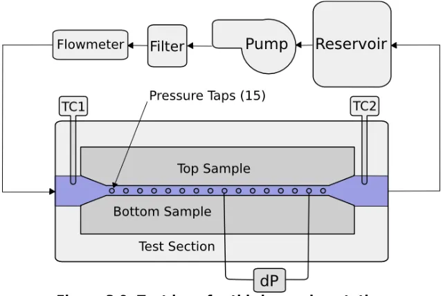
The test section is rectangular in shape, with a fixed width of 12.2 mm

(0.48in) and a variable height, fixed by four set screws. The test section is

88.9 mm (3.5 in) long and has static pressure taps along the length of the

channel. These taps are spaced 6.35 mm (0.25 in) apart for a total of 16

taps along the channel length, and are formed with a #60 drill (diameter

= 1.016 mm) in the wall of aluminum. Care was taken to leave no burrs

protruding into the flow. The taps are all connected to a pressure

manifold, with a separate valve for each tap. At the end of the pressure

manifold is a Honeywell 0-690 kPa (0-100 psi) differential pressure sensor

powered by an Electro Industries Laboratory DC power supply. At the

inlet and outlet, two K type thermocouples measure the temperature of

the water. To control the separation, two Mitutoyo Digimatic Micrometer

heads with ±2.54 μm accuracy are used to set the separation, which is

then fixed in place with screws.

The pressure sensor is connected to one channel of a simple LM324

operational amplifier circuit, with the gain set at 67. The design used is a

basic non-inverting amplifier circuit. The op-amp circuit is powered by an

Electro Industries Laboratory DC power supply (at +31VDC). The amplified

voltage reading is calibrated to a pressure using an OMEGA DPS-610

Pressure calibrator. Pressure readings are then obtained using the

voltage recorded by a Craftsman 82040 Multimeter.

3.2.2 Experimental Schematics and Drawings

A simple schematic of the setup can be seen in Figure 3.1.

The test section itself was machined from 6061 aluminum stock. An

exploded view of the test section makeup is given in Figure 3.2.

In Figure 3.2 the two red blocks are the samples that form the

microchannel. The yellow block on the top holds the top sample fixed.

The yellow block on the bottom holds 2 screws and 2 micrometer

positioning heads that allow the separation of the setup to be varied. This

allows the same samples to be used in channels of varying diameters,

essentially varying the relative roughness. The blue piece comprises one

3 Experimental Work - 3.2 Initial Experimental Work – Sawtooth High Page 48

Figure 3.2: Left: Exploded view of the setup Right: Assembled setup without cover piece

wall of the channel and features pressure taps for measuring static

pressure along the channel. The end of the channel is made up of the

light blue piece. Finally, the green cover comprises another wall, and

holds the inlet and outlet of the channel.

3.2.3 Samples used in First Experimentation

With this setup, the effects of sawtooth roughness with high relative

roughness was examined. Two sample sets were used for the roughened

channels. They had similar roughness heights, but differed in the pitch of

the roughness elements. First however, the experimental setup is

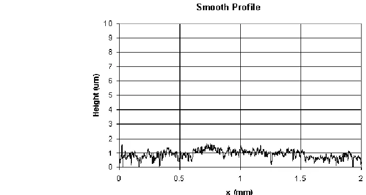
validated using samples that were ground to be flat and smooth. The

smooth channel profile as obtained by a stylus profilometer can be seen

in Figure 3.5. The height of roughness from the grinding process is

around ε=2 μm. The values obtained from these smooth channel tests

are expected to match theoretical values for smooth rectangular

channels.

Two different sample sets were machined using a ball end mill of

appropriate diameter. The ball end mill was run perpendicular to the test

samples to machine grooves at a shallow depth. The ball end mill

diameter was 762 μm.

3 Experimental Work - 3.2 Initial Experimental Work – Sawtooth High Page 49

Table 3.1: Summary of Roughness in First Experimentation

Pitch Ra Fp

μm μm μm μm

Smooth N/A 2 0.31 N/A

405 99.71 27.43 23.34

815 105.55 24.19 21.52

ε_FP

For this experiment, two pitches of 415 μm and 815 µm were employed.

The profile of the p=415 μm sample is shown in Figure 3.3, and was

obtained with a Mitutoyo stylus profilometer. It can be seen from

measuring eight different parts of the sample in 2 mm samples that the

height of the roughness elements are ε = 99.71 μm. The 815 μm pitch

sample had a roughness profile that is shown in Figure 3.4. Every other

roughness element on these samples was machined somewhat

3 Experimental Work - 3.2 Initial Experimental Work – Sawtooth High Page 50

Figure 3.4: 815um pitch profile, taken with stylus profilometer

differently. Only the tops of every other element were removed, rather

than the entire element. On these samples the height of the roughness

elements is ε=105.55 μm.

The geometries of the samples are summarized in Table 3.1. The value of

Ra is calculated from the raw profilometer data by averaging the heights

according to ASME standards. The value of Fp was then obtained with a

simple program that ignored all data above Ra and found the average of

the rest of the data. Fp is then the distance from the average roughness

to the floor profile line.

3 Experimental Work - 3.2 Initial Experimenta