A cartesian-grid integrated-RBF method for viscoelastic flows

This article has been downloaded from IOPscience. Please scroll down to see the full text article.

2010 IOP Conf. Ser.: Mater. Sci. Eng. 10 012210

(http://iopscience.iop.org/1757-899X/10/1/012210)

Download details: IP Address: 139.86.2.14

The article was downloaded on 06/07/2010 at 08:19

Please note that terms and conditions apply.

A Cartesian-grid integrated-RBF method for

viscoelastic flows

D. Ho-Minh, N. Mai-Duy and T. Tran-Cong Computational Engineering and Science Research Centre (CESRC), Faculty of Engineering and Surveying (FoES),

The University of Southern Queensland (USQ), Toowoomba, QLD 4350, Australia

E-mail: [email protected]

Abstract. This paper is concerned with the use of integrated radial-basis-function networks (IRBFNs), Cartesian-grids and point collocation for numerically solving 2D flows of viscoelastic fluids. In the proposed method, RBFNs, which are constructed through integration, are employed to approximate the field variables including stresses, and the governing equations are discretised by means of point collocation. Advantages gained from the integration process over differentiated RBFNs process are (i) better accuracy (ii) more straightforward implementation of boundary conditions and (iii) more stable solutions. The method is verified through several test problems, e.g. planar Poiseuille flow and fully-developed flow in a square duct, with different types of viscoelastic fluids, namely Oldroyd-B and CEF. The obtained results show that (i) The proposed method is easy to implement; (ii) Its pre-processing is simple and (iii) Accurate results are obtained using relatively-coarse grids.

1. Introduction

Radial-basis-function networks (RBFNs) have been shown to be a powerful numerical tool for the solution of partial-differential equations (PDEs). The first report on this subject was made by Kansa [1]. For Kansa’s method, a function is first represented by an RBFN which is then differentiated to obtain approximate expressions for its derivative functions. On the other hand, to avoid the reduction in convergence rate caused by differentiation, Mai-Duy and Tran-Cong [2] proposed an indirect/integrated RBFN (IRBFN) approach in which the highest-order derivatives in the PDE are first decomposed into RBFs, and their lower-order derivatives and the function itself are then obtained through integration. Previous studies (e.g. [2]) showed that IRBFN collocation methods yield better accuracy than differentiated RBFN (DRBFN) ones for both the representation of functions and the solution of PDEs.

grids, is applied to simulate fully developed flows between two parallel planes and in rectangular ducts. Results obtained show that good agreement with data available in the literature is achieved using relatively coarse grids.

The remainder of this paper is organised as follows. Governing equations are summarised in Section 2. Section 3 presents the proposed integrated-RBF method. Two test problems are simulated in Section 4. Section 5 concludes the paper.

2. Governing equations

In the case of an incompressible fluid, the equations for the conservation of momentum and mass take the forms

ρ

∂v

∂t +v· ∇v

= ∇ ·σ+f x∈Ω, (1)

∇ ·v = 0 x∈Ω, (2)

where v is the velocity vector,f the body force per unit volume of fluid, ρdensity, σ the stress tensor (Cauchy stress tensor),t the time, xthe position vector and Ω the domain of interest. The stress tensor can be decomposed into

σ=−pI +τ, (3)

where p is the pressure, I the unit tensor and τ the extra stress tensor. In this paper, the working fluids are the CEF and the Oldroyd-B with the extra stress tensors defined as

τ = 2η(d)d−ψ₁ ∇

d+4ψ₂d.d (CEF model), (4)

τ = 2ηs(

λ₂ λ1

)d+τv (Oldroyd−B model), (5)

with

τv+λ1

∇

τv = 2ηv(1−

λ₂ λ1

)d, (6)

where dis the rate of deformation tensor

d= 1

2(∇v+ (∇v)

T_{); (7)}

dis the scalar magnitude of d

d=p2tr(d.d); (8)

in which ‘tr′

denotes the trace operation; Ψ1 and Ψ2 the first and the second normal stress

coefficients, respectively; ηs the solvent viscosity; τv is the extra stress due to viscoelasticity;

λ1 and λ2 are characteristic relaxation and retardation times of the fluid, respectively; ηv is the

zero shear polymer viscosity and

∇

[ ] the upper convected derivative defined as

∇

[ ]= ∂[ ]

∂t +v· ∇[ ]−(∇v)

T _.

[ ]−[ ]· ∇v. (9)

3. Proposed 1D-RBFN technique

In the present technique, point collocation is applied to reduce the PDEs to sets of algebraic equations. The problem domain is represented by a Cartesian grid. Since the governing equations are of second order, the integral RBF scheme of second order is ustilised here. IRBFN expressions on the x and y grid lines have similar forms. In the following, only a x grid line is considered. On the grid line, a functionf and its derivatives with respect toxcan be represented as follows

d2f(x) dx2 =

Nx

X

i=1

wigi(x) = Nx

X

i=1

wiI_i(2)(x), (10)

df(x)

dx =

Nx

X

i=1

wiIi(1)(x) +c1, (11)

f(x) =

Nx

X

i=1

wiI_i(0)(x) +c1x+c2, (12)

where Nx is the number of nodes on the grid line, {wi}N_i=1x the set of network weights,

{gi(x)}Ni=1x ≡

n

I_i(2)(x)oNx

i=1 the set of RBFs, I (1)

i (x) =

R

I_i(2)(x)dx, I_i(0)(x) = R I_i(1)(x)dx, and c1 and c2 are the constants of integration.

Evaluation of (10) - (12) at the grid nodes leads to

d

d2_f

dx2 = Ib

(2)_{α,b (13)}

b

df

dx = Ib

(1)_{α,b (14)}

b

f = Ib(0)α,b (15)

where the superscript (.) is used to denote the order of the corresponding derivative function;

b

I(2) =

     

I₁(2)(x₁), I₂(2)(x₁), · · ·, I_N(2)

x(x1), 0, 0

I₁(2)(x2), I2(2)(x2), · · ·, IN(2)x(x2), 0, 0

..

. ... . .. ... ... ... I₁(2)(xNx), I

(2)

2 (xNx), · · ·, I

(2)

Nx(xNx), 0, 0

    

; (16)

b

I(1) =

     

I₁(1)(x1), I2(1)(x1), · · ·, IN(1)x(x1), 1, 0

I₁(1)(x2), I₂(1)(x2), · · ·, I_N(1)x(x2), 1, 0

..

. ... . .. ... ... ... I₁(1)(xNx), I

(1)

2 (xNx), · · ·, I

(1)

Nx(xNx), 1, 0

    

; (17)

b

I(0) =

     

I₁(0)(x₁), I₂(0)(x₁), · · ·, I_N(0)

x(x1), x1, 1

I₁(0)(x2), I2(0)(x2), · · ·, IN(0)x(x2), x2, 1

..

. ... . .. ... ... ...

I₁(0)(xNx), I

(0)

2 (xNx), · · ·, I

(0)

Nx(xNx), xNx, 1

    

; (18)

b

α = (w1, w2,· · ·, wNx, c1, c2) T

in which d fj dx =d f(xj) dx and fj =f(xj) withj ={1,2,· · ·, Nx}. It is noted thatf is

used to represent the field variables, e.g. the component of v, in (1)–(6).

4. Numerical results

This section presents the verification of the proposed method with the simulation of the planar Poiseuille flow and fully-developed viscoelastic flow in rectangular ducts. Fluids models considered are Oldroyd-B and CEF. Uniform grids are used to represent the problem domain, and 1D-IRBFNs are implemented with the multiquadric (MQ) function

gi(x) =

q

(x−ci)2+a2_i, (22)

where ci and ai are the centre and the width/shape-parameter of the ith MQ-RBF. The MQ

width is simply chosen to be the grid size.

0 0.2 0.4 0.6 0.8 1

0 0.2 0.4 0.6 0.8 1 1.2 1.4

y

v

analytic x=0.5

Figure 1. Steady-state planar Poiseuille flow using Oldroyd-B model: the velocity on the middle planex= 0.5 with 31×31 collocation points.

4.1. Planar Poiseuille flow

First, planar Poiseuille flow that has an analytical solution is considered. The governing equations with Oldroyd-B model in dimensionless form are given by

∇ ·v = 0, (23)

∂v

∂t +v· ∇v = − 1 Re∇p+

1 Reτv+

β

Re∆v, (24)

τv+W e ∇

τv = 2 (1−β)d, (25)

where W e is the Weissenberg number,Re the Reynolds number and β the ratio of retardation and relaxation times of the fluid (its value is taken to be 1/9 in this work).

A unit domain, [0,1]×[0,1], is taken as a computational domain. On the solid boundaries (y= 0 andy= 1), non-slip conditions are imposed. At the steady-state condition, the velocity and stress fields are given in the following analytic forms

vx = 4 (1−y)y, (26)

vy = 0, (27)

τxx = 2W e(1−β)

∂vx

∂y

2

, (28)

τyy = 0, (29)

τxy = (1−β)

∂vx

∂y

. (30)

In solving (23)–(25), the material derivatives are approximated using an Euler scheme

∂G

∂t +v· ∇G≈

Gn+1−Gn ∆t +v

n_{· ∇G}n ₍₃₁₎

in which Grepresentsv andτ, and the deformation term is treated explicitly

∇v·τ+τ ·(∇v)T ≈ ∇vn·τn+τn·(∇vn)T . (32)

The solution procedure can be outlined as follows

• Calculation of intermediate velocity v∗ from the momentum equation (24), where the pressure term is removed. At the beginning, the inlet velocity is chosen to be zero or takes a parabolic profile as in (26),

• Calculation of pressure from the continuity equation (23)

∆p= Re ∆t∇ ·v

∗

, (33)

• Correction of intermediate velocity using the computed pressure just obtained

vn+1 =vn−∆t

Re∇p

n+1_{, (34)}

• Calculation of viscoelastic stress components from the constitutive equation (25),

• Re-imposition of inlet velocity profile using the obtained outlet velocity profile,

• Repeating the above steps until there is no further change (above a given small tolerance) in the outlet velocity profile.

0 0.2 0.4 0.6 0.8 1 0

20 40 60

y

τ

We=2

We=1

We=0.5 We=0.1

0 0.2 0.4 0.6 0.8 1

−4 −3 −2 −1 0

y

τ

Figure 2. Steady-state planar Poiseuille flow using Oldroyd-B model: a) the first normal stress difference (N1 = τxx −τyy = τxx) and b) the shear stress on the middle plane x = 0.5 with

31×31 collocation points at different values of theW e number.

a) b)

c)

d)

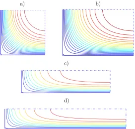
Figure 3. Flow in rectangular ducts: Streamlines of secondary flows in one quarter of the cross-section with the aspect ratios of a) 1, b) 1.56, c) 4 and d) 6.25 using a grid of 41×41.

a) b)

c)

d)

Figure 4. Flow in rectangular ducts: Contour plots for the vorticity ω in one quarter of the cross-section at four different aspect ratios: a) 1, b) 1.56, c) 4 and d) 6.25 using a grid of 41×41.

a) b)

c)

d)

Figure 5. Flow in rectangular ducts: Contour plots for the primary velocity vz in one quarter

c)

d)

Figure 6. Flow in rectangular ducts: Contour plots for the second normal stress difference (N2 =τxx−τyy) in one quarter of the cross-section at four different aspect ratios: a) 1, b) 1.56,

c) 4 and d) 6.25 using a grid of 41×41.

4.2. Fully-developed viscoelastic flow in rectangular ducts

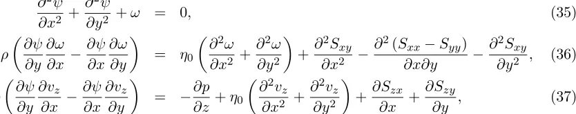
The flow of a viscoelastic fluid in a rectangular duct has received a great deal of attention because of its fundamental and practical importance. Many studies were carried out on this geometry with different constitutive models, (e.g. Reiner-Rivlin [7], CEF [8, 9] and modified PTT (MPTT) [10]). Results by Gervang and Larsen [8], where both numerical and experimental investigations were conducted, are often cited in the literature. The governing equations are taken in terms of stream-function, vorticity and primary velocity

∂2ψ ∂x2 +

∂2ψ

∂y2 +ω = 0, (35)

ρ ∂ψ ∂y ∂ω ∂x − ∂ψ ∂x ∂ω ∂y

= η₀

∂2ω ∂x2 +

∂2ω ∂y2

+∂

2_S

xy

∂x2 −

∂2(Sxx−Syy)

∂x∂y −

∂2Sxy

∂y2 , (36)

ρ ∂ψ ∂y ∂vz ∂x − ∂ψ ∂x ∂vz ∂y

= −∂p

∂z +η0

∂2vz

∂x2 +

∂2vz

∂y2

+∂Szx ∂x +

∂Szy

∂y , (37)

with the homogeneous boundary conditions for ψ, ∂ψ/∂n and vz. A CEF fluid is considered.

The computation boundary conditions for the vorticity in (36) can be derived from the stream-function equation. The process is similar to that in [6]. Equations (35)–(37) are thus subject to Dirichlet boundary conditions. The flows are generated by pressure drop ∂p/∂z. The stress components are directly computed from the velocity field using (4). Unlike the planar Poiseuille flow problem, a Picard iterative scheme is applied here to solve the resultant system of nonlinear algebraic equations. Figures (3)- (6) show the patterns of the primary and secondary flows together with the second normal stress difference for different aspect ratios 1, 1.56, 4 and 6.25.

Since the flow is symmetric about the vertical and horizontal centreline, only one quarter of the cross-section is plotted. Each quadrant has two vortices, whose pattern and strength strongly depend on the aspect ratio for a given mean primary velocity. The two vortices are symmetric about the diagonal plane in the case of ratio 1. For aspect ratio greater than 1, the vortex near the long wall moves towards the short wall while the vortex near the short wall is reduced with increasing aspect ratios. The results are similar to those reported in the literature (e.g. [8, 10]).

5. Concluding remarks

Fully-developed flows of viscoelastic fluids between two parallel walls and in rectangular ducts were studied with the IRBFN collocation technique. The calculations are carried out in both the primitive variable and the stream-function–vorticity formulations. The technique is easy to implement. Results obtained are in good agreement with the exact solution and those by other techniques. Extension of the proposed method to viscoelastic flows is underway and new results will be reported in future.

Acknowledgments

This research is supported by Australia Research Council and FoES-USQ. D. Ho-Minh would like to thank the CESRC, FoES and USQ for a postgraduate scholarship.

References

[1] Kansa E J 1990 Computers and Mathematics with Applications 19127–145 [2] Mai-Duy N and Tran-Cong T 2001Neural Networks14_185–199

[3] Schaback R 1995Advances in Computational Mathematics 3251–264

[4] Mai-Duy N and Tran-Cong T 2007Numerical Methods for Partial Differential Equations 23_1192–1210 [5] Mai-Duy N and Tran-Cong T 2009Engineering Analysis with Boundary Elements 33191–199

[6] Ho-Minh D, Mai-Duy N and Tran-Cong T 2009CMES 44219–248 [7] Green G and Rivlin R 1956Quaterfly of Applied Mathematics 14299–308

[8] Gervang B and Larsen P 1991Journal of Non-Newtonian Fluid Mechanics39217–237

[9] Mai-Duy N and Tanner R I 2007 International Journal of Numerical Methods for heat & fluid flows 17 165–186