Continuous-time random walks on networks with vertex- and time-dependent forcing

Continuous-time random walks on networks with vertex- and time-dependent forcing

C. N. Angstmann,*I. C. Donnelly,†and B. I. Henry‡

School of Mathematics and Statistics, University of New South Wales, Sydney, New South Wales 2052, Australia

T. A. M. Langlands§

Department of Mathematics and Computing, University of Southern Queensland, Toowoomba, Queensland 4350, Australia (Received 28 June 2013; published 20 August 2013)

We have investigated the transport of particles moving as random walks on the vertices of a network, subject to vertex- and time-dependent forcing. We have derived the generalized master equations for this transport using continuous time random walks, characterized by jump and waiting time densities, as the underlying stochastic process. The forcing is incorporated through a vertex- and time-dependent bias in the jump densities governing the random walking particles. As a particular case, we consider particle forcing proportional to the concentration of particles on adjacent vertices, analogous to self-chemotactic attraction in a spatial continuum. Our algebraic and numerical studies of this system reveal an interesting pair-aggregation pattern formation in which the steady state is composed of a high concentration of particles on a small number of isolated pairs of adjacent vertices. The steady states do not exhibit this pair aggregation if the transport is random on the vertices, i.e., without forcing. The manifestation of pair aggregation on a transport network may thus be a signature of self-chemotactic-like forcing.

DOI:10.1103/PhysRevE.88.022811 PACS number(s): 05.10.Gg, 05.40.Fb, 89.75.Kd

I. INTRODUCTION

Stochastic transport on networks is present in diverse fields including contagion through passenger transport [1,2], CO2 sequestration in porous media [3], and spatial progression of dementia in the brain [4]. It is natural to consider pattern forma-tion, characterized by a buildup of concentration on selected vertices, in such systems since pattern formation signatures may contain useful information about the functioning of the network. In a spatial continuum, pattern formation arising from stochastic transport with reactions or forcing has been widely studied [5]. However, the study of pattern formation for stochastic transport on a network with reactions or forcing is a recent field of study [6–12].

A useful model for studying stochastic transport of particles on a spatial continuum or a regular lattice is the continuous time random walk (CTRW) [13,14], in which a particle waits for a random time before randomly jumping to a new location. This process is defined by a waiting time density and a jump density. In a recent paper, we started with this model as the underlying stochastic process and derived the generalized master equations for random motion of particles between vertices on a network, with reaction dynamics localized on the vertices [12]. This enabled us to study pattern formation on transport networks with reactions. In this paper, we use a similar approach to study pattern formation on transport networks with forcing, but without reactions.

One way of introducing the effect of a force field into a CTRW is by including a bias in the jump density [15–17]. A variety of force fields may be modeled with this approach. Examples include subdiffusion with a constant force field

*_{[email protected]}

†_{[email protected]} ‡_{[email protected]} §_{[email protected]}

[18], subdiffusion with advection [19], and subdiffusion with chemotaxis [20]. Chemotaxis refers to the directed migration of particles along a gradient of chemokines [21–26]. Self-chemotaxis corresponds to the case where the particles are themselves the chemokines. The inclusion of a self-chemotactic force leads to an aggregation of particles due to the flux of particles being continually directed towards regions of higher concentration. A self-chemotactic-like (SCL) forcing can be introduced in a CTRW model for transport on a network by biasing the jump density of a randomly walking particle towards adjacent vertices with higher concentrations of particles.

Subdiffusion is a form of anomalous diffusion where the mean squared displacement increases as a fractional power

α <1 of time, i.e.,x2_{(t) ∼t}α_{[27]. Both standard diffusion}

and subdiffusion [28–31] may be modeled with CTRWs by including exponential or power law waiting time densities, respectively [27]. There have been numerous studies of pattern formation in subdiffusive systems on a spatial continuum [16,32–34]. Of particular interest to the studies below is anomalous aggregation, which occurs in systems with spatially variant power law waiting time densities. The anomalous aggregation occurs at the spatial location with the lowest power law exponent [16,35].

Here we derive a set of generalized master equations governing the CTRW transport of particles on a network, subject to a vertex- and time-dependent force field. As a particular case, we consider a transport network with all particles of the same species and SCL forcing. We have carried out simulations for both exponential and Mittag-Leffler waiting time densities on a 50 vertex Watts-Strogatz network [36].

state pattern seen in unforced systems [12] and it occurs in systems with either exponential or Mittag-Leffler waiting time densities. The pair aggregation is also very different from the anomalous aggregation that we observe with a Mittag-Leffler waiting time density on a single vertex and exponential waiting time densities on the remaining vertices.

II. DERIVATION OF A CTRW NETWORK GENERALIZED MASTER EQUATION

A network is defined as a set of vertices connected by a set of edges. The network topology is completely defined by its adjacency matrix,

Ai,j =

1 if there is an edge between vertexiand vertexj

0 otherwise .

(1) Particles moving at random between connected vertices of a network may be modeled as CTRWs. Here we consider a general case where the waiting time density may be different on different vertices and the effects of a force field are incorporated by biasing the probability of jumping to different connected vertices. This bias may be vertex and time dependent. To derive the generalized master equations for this process, we follow the derivation of the master equation for CTRWs on a spatial continuum carried out in [15,17].

We now consider the behavior of a single particle traversing across a network withJvertices. The probability flux density for the particle to arrive at a vertexvi, at timet, after taking njumps, given the particle began at vertexv₀, at timet =t₀, is [14]

qn₊1(vi,t|v0,t0)=

J

j=1

t

t0

(vi,t|vj,t)qn(vj,t|v0,t0)dt.

(2) Here,(vi,t|vj,t) is the probability density for jumping to

vi att, conditional on arrival atvj at the earlier timet. The assumed initial condition for the particle is

q0(vi,t|v0,t0)=δvi,v0δ(t−t +

0). (3) To find the total probability flux density for arrivals atviatt, we sum over the number of jumps,

q(vi,t|v0,t0)= ∞

n=0

qn(vi,t|v0,t0). (4)

This then yields

q(vi,t|v0,t0)=

J

j=1

t

t0

(vi,t|vj,t)q(vj,t|v0,t0)dt

+δv_i,v0δ(t−t +

0 ). (5)

We assume that the transition density,(vi,t|vj,t), may

be expressed as

(vi,t|vj,t)=λ(vi|t,vj)ψ(t−t|vj), (6)

where λ and ψ are the independent jump and waiting time densities, respectively. The network jump density, from

vj to vi, incorporates the topology of the network, i.e.,

λ(vi|t,vj)=0 if Aj,i=0. The densities satisfy the nor-malizations Ji=1λ(vi|t,vj)=1 for given vj and t and

_∞

0 ψ(τ|vj)dτ =1 for givenvj.

The probability density of a particle being atvi at timet, conditional on the particle starting atv0at timet =t0, is

ρ(vi,t|v0,t0)=

t

t0

(t−t|vi)q(vi,t|v0,t0)dt. (7)

Here, (t−t|vi)=1−₀t−tψ(τ|vi)dτis the survival prob-ability function of a particle not jumping fromvi before time

t, given it arrived atviat the earlier timet.

Taking care of the singularity due to the initial conditions, we first define [17,37]

q(vi,t|v0,t0)=δvi,v0δ(t−t +

0)+q+(vi,t|v0,t0), (8) where

q+(vi,t|v0,t0)=

J

j=1

t

t0

(vi,t|vj,t)q(vj,t|v0,t0)dt (9)

is right side continuous at t =t0. Substituting Eq. (8) into Eq.(7)and differentiating yields

dρ(vi,t|v0,t0)

dt =q

+_(v

i,t|v0,t0)−δvi,v0ψ(t−t0|vi)

−

t

t0

q+(vi,t|v0,t0)ψ(t−t|vi)dt. (10)

Further substituting Eq.(9), with Eq.(8), into Eq.(10)yields

dρ(vi,t|v0,t0)

dt

=

J

j₌1

λ(vi|t,vj)

t

t0

ψ(t−t|vj)q(vj,t|v0,t0)dt

−

t

t0

ψ(t−t|vi)q(vi,t|v0,t0)dt. (11)

We can express the right-hand side of the above in terms ofρ

by introducing a memory kernel,K(t|vi), defined by

t

t0

ψ(t−t|vi)q(vi,t|v0,t0)dt

=

t

t0

K(t−t|vi)

t

t0

(t−t|vi)q(vi,t|v0,t0)dt

dt

=

t

t0

K(t−t|vi)ρ(vi,t|v0,t0)dt. (12)

This equivalently defines the memory kernel asL{K(t|vi)} =

L{ψ(t|vi)}/L{ (t|vi)}, where L denotes the Laplace trans-form with respect to time.

We now move from considering the behavior of a single particle to that of an ensemble of particles. We define the density of an ensemble of particles at vertexvi at timet to be

u(vi,t)=

v0∈V

t

t0

ρ(vi,t|v0,t0)dt0, (13)

whereV is the set of all vertices. Then, by substituting Eq.(12)

ensemble generalized master equations for stochastic transport on a network with vertex- and time-dependent forcing:

du(vi,t)

dt =

J

j=1

λ(vi|t,vj)

t

t0

K(t−t|vj)u(vj,t)dt

−

t

t0

K(t−t|vi)u(vi,t)dt, i=1, . . . ,J.

(14) The forcing is incorporated through the vertex- and time-dependent bias in the jump densities. In the simplest case, stochastic transport on a network can be modeled by having the probability of jumping between connected vertices equal (equal edge weights). Equation (14) provides a model for stochastic transport on a network with time-dependent edge weightings.

A. Self-chemotactic-like forcing

Self-chemotactic-like (SCL) forcing can be included in Eq. (14) through a bias in the jump density dependent on the concentration of particles on neighboring vertices. By analogy with the standard form for chemotactic attraction in the continuum [38], we consider jump densities of the form

λ(vi|t,vj)=

Aj,ieβu(vi,t)

J

k₌1Aj,keβu(vk,t)

. (15)

The factoreβu(vi,t)_{is a sensitivity function that depends on the} concentration of the attractantu(vi,t) and the strength of the

chemotaxis,β[38].

The generalized master equations with SCL forcing are thus given by

du(vi,t)

dt =

J

j₌1

Aj,ieβu(vi,t)

J

k=1Aj,keβu(vk,t)

t

t0

K(t−t|vj)u(vj,t)dt

−

t

t0

K(t−t|vi)u(vi,t)dt, i=1, . . . ,J.

(16)

III. NUMERICAL SIMULATIONS

In the simulations below, we consider a Watts-Strogatz (WS) network with 50 vertices and rewiring probability of

p=0.05 [36]. This class of random network is a widely used model, in part due to the property of low graph diameter, which is a feature seen in metabolic [39], functional brain [40], and

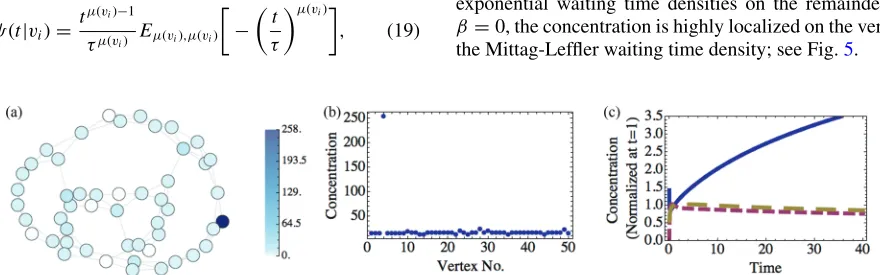
FIG. 1. (Color online) (a) Concentration of particles att=10 000 on network and (b) distribution of concentration, for a 50 vertex Watts-Strogatz network with rewiring probabilityp=0.05 and exponential waiting time densities.

FIG. 2. (Color online) (a) Concentration of particles att=10 000 on network and (b) distribution of concentration, for a 50 vertex Watts-Strogatz network with rewiring probabilityp=0.05 and with vertex-dependent exponential waiting time densities.

genomic [41] networks. For consistency in evaluating changes in parameters, the same random initial condition is used for all numerical simulations. We have explored WS networks with different numbers of vertices, different rewiring probabilities, and different initial conditions, and the qualitative behavior of pair aggregation, reported below, is consistent across these changes.

A. Exponential waiting time densities

We first consider CTRWs on the network with exponential waiting time densities,

ψ(t|vi)=γ(vi)e−γ(vi)t_{. (17)} In this case, it can be shown thatK(t|vi)=γ(vi)δ(t) [17], and Eq.(16)is now

du(vi,t)

dt =

J

j=1

Aj,ieβu(vi,t)

J

k=1Aj,keβu(vk,t)

γ(vj)u(vj,t)

−γ(vi)u(vi,t), i=1, . . . ,J. (18)

If there is no SCL forcing,β =0, and ifγ(vi)=γ for allvi, then we recover the unforced Case A Laplacian, previously introduced in [12]. The steady state concentration for this system is proportional to vertex degree, i.e.,u(vi,t)∝κiwhere κi=

J

j=1Ai,j is the number of edges connecting tovi.

If there is SCL forcing in this system, β >0, then the steady state concentration is characterized by pair aggregation in which distinct pairs of adjacent vertices have high concen-tration and other vertices having essentially no concenconcen-tration. Figure1shows the case whenβ =1 andγ(vi)=1 for alli.

In the Appendix, we formally show that pair aggregation is a linearly stable steady state solution of Eq.(18).

0.0 0.2 0.4 0.6 0.8 1.0 0

2 4 6 8

β

N

o

. o

f

P

a

irs

FIG. 4. (Color online) (a) Concentration of particles att=400 on network and (b) distribution of concentration, for a 50 vertex Watts-Strogatz network with rewiring probabilityp=0.05 and Mittag-Leffler waiting time densities. (c) The concentration as a function of time on vertices 4 (continuous line) and 6 (dashed line). These concentrations are normalized to the concentration att=10.

When there is SCL forcing and the rate parameter in the waiting time density is chosen differently for each vertex, the steady state concentration is characterized by distinct pairs of adjacent vertices having high, but unequal, concentration and other vertices having essentially no concentration. An example of this is shown in Fig.2. The steady state in this case is char-acterized by unequal concentrations within each pair through the relationu(vi,t)γ(vi)=u(vj,t)γ(vj). In the Appendix, this is algebraically shown to be a stable, steady state solution of the generalized master equations, given by Eq.(18).

To investigate the effects of the strength of the chemoattrac-tive sensitivity function given in Eq.(18), we have carried out numerical simulations for a range ofβ ∈[0,1000]; see Fig.3. Forβ =0, the steady state concentration on each vertex is linearly dependent on vertex degree [12]. For sufficiently small

β >0, the steady state changes but there is no aggregation onto pairs of connected vertices. As β is increased, the number of pairs of vertices with high concentration increases monotonically. The critical values of β, below which there are no pairs, and above which the number of pairs no longer increases with increasing β, are dependent on both the initial conditions and the network topology. However, between the critical values, the number of pairs still increases monotonically withβ.

B. Mittag-Leffler waiting time densities

We now consider CTRWs on the network with Mittag-Leffler waiting time densities [42],

ψ(t|vi)= tμ(vi)−1

τμ(vi) Eμ(vi),μ(vi)

− t

τ

μ(vi)

, (19)

for 0< μ(vi)<1. In this equation, τ is a constant scale

parameter,μ(vi) is a vertex-dependent scaling exponent, and

Eζ,ξ(t)= ∞

n=0

tn (ζ n+ξ)

is the generalized Mittag-Leffler function. The waiting time density defined by Eq. (19) is a heavy tailed function with power law decay of the formt−1+μ(vi)_{. The generalized master} equations, Eq.(16)in this case, can be written as

du(vi,t)

dt =

J

j=1

Aj,ieβu(vi,t)

J

k=1Aj,keβu(vk,t) 1

τμ(vj)₀D 1−μ(vj) t u(vj,t)

− 1

τμ(vi)₀D 1−μ(vi)

t u(vi,t), i=1, . . . ,J, (20)

where the memory kernel is given by the relation in Laplace spaces;L{K(vi,s)} ∼ 1

τμ(vj)s

1−μ(vi)_and

0Dt1−μis a

Riemann-Liouville fractional derivative [43].

Figure 4 shows the simulation of Eq. (20) with β =1. The pair aggregation is very similar but not identical to the pair aggregation with exponential waiting time densities; see Fig.1.

In the Appendix, we have carried out linear stability analysis of paired steady states and we have shown that these classes of steady states are linearly stable. The approach to the steady state is shown in Fig.4(c).

We have also carried out a range of simulations with a Mittag-Leffler waiting time density on a selected vertex and exponential waiting time densities on the remainder. When

β =0, the concentration is highly localized on the vertex with the Mittag-Leffler waiting time density; see Fig.5.

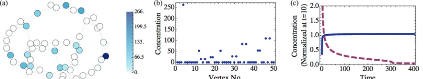
FIG. 6. (Color online) (a) Concentration of particles att=400 on network and (b) distribution of concentration, for a 50 vertex Watts-Strogatz network with rewiring probabilityp=0.05 withβ=1. (c) The concentration as a function of time on vertices 4 (continuous line) and 5 (dashed line). These concentrations are normalized to the concentration att=10. Vertex 4 has an Mittag-Leffler waiting density, while the rest of the vertices have identical exponential waiting time densities.

This is similar to the anomalous aggregation observed in the continuum [16,35]. The increase in concentration at the site with the Mittag-Leffler waiting time density and the decay in concentration at other vertices is shown in Fig.5(c). If the SCL forcing is included, then pair aggregation occurs, except in the neighborhood of the vertex with the Mittag-Leffler waiting time density. The anomalous aggregation can be seen at vertex 4 of Fig.6(b), with pair aggregates or essentially zero concentrations on the rest of the vertices. The approach to the steady state is shown in Fig.6(c)for the vertex with the Mittag-Leffler waiting time density and a neighboring vertex with exponential waiting time densities.

IV. CONCLUSION

We have considered the problem of particles moving randomly from vertex to vertex on a network, with a bias due to a force field that varies across the vertices and in time. The problem is formulated using a continuous time random walk as the underlying stochastic process, and the generalized master equations for the concentration of particles on vertices have been derived. The generalized master equations also allow for the modeling of networks with weighted edges, where the edge weights may be a function of time. From this general model, we consider the particular case of stochastic transport on a network with a self-chemotactic-like force. With this force, the jump densities of the particles are biased so that they are more likely to jump to neighboring vertices that have higher concentrations of particles. We have carried out an algebraic linear stability analysis of steady state solutions and we have performed numerical simulations over a range of strengths of the chemotactic attraction. The stochastic transport with self-chemotactic-like forcing results in pair-aggregate pattern formation in which particles pair-aggregate onto distinct pairs of connected vertices. We considered two different waiting time densities in our analysis: an exponential waiting time density and a Mittag-Leffler waiting time density. On a spatial continuum, these waiting time densities result in standard diffusion and subdiffusion, respectively. The aggregation from self-chemotactic-like forcing persists for systems with either of these waiting time densities. The pair aggregation can also coexist with anomalous aggregation, caused by having a power law waiting time density on a single vertex and having exponential waiting time densities on the remainder.

ACKNOWLEDGMENT

This work was supported by the Australian Commonwealth Government (Grant No. ARC DP1094680).

APPENDIX: LINEAR STABILITY ANALYSIS

In this Appendix, we show that pair aggregation is a linearly stable steady state solution of the generalized master equations for both exponential and Mittag-Leffler waiting time densities, given by Eqs.(18)and(20). A pair-aggregate steady state is defined as two connected vertices,u(vm,t) andu(vn,t), with a high concentration and the remainingu(vi,t)=0. This steady state is exact in the limitu(vm,t)→ ∞andu(vn,t)→ ∞; and

u(vi,t)≈0 for large, but finiteu(vm,t) andu(vn,t).

1. Exponential waiting time densities

The generalized master equations with SCL forcing and exponential waiting time densities are given by

du(vi,t)

dt =

J

j=1

Aj,ieβu(vi,t)

J

k=1Aj,keβu(vk,t)

γ(vj)u(vj,t)

−γ(vi)u(vi,t), i=1, . . . ,J. (A1)

Here we consider a single pair aggregation, defined as

γ(vm)u(vm,t)=γ(vn)u(vn,t) with the remainingu(vi,t)=0, and show that it is an approximate linearly stable steady state solution of the generalized master equations, given by Eq.(A1) for sufficiently large, constantu(vm,t) and u(vn,t).

For notational simplicity, we writeu(vi,t) asuiandγ(vi)=γi.

Note also that

J

k=1

Am,keβuk = J

k=1,k=n

Am,keβ0+eβun

=κm−1+eβun, (A2)

J

k=1

An,keβuk = J

k=1,k=m

An,keβ0+eβum

=κn−1+eβum_{, (A3)}

whereκiis the degree ofvi. For constantui, the left-hand side

For vertices i=m,n, the right-hand side of Eq. (A1)

simplifies to

Am,iγmum

J

k₌1Am,keβuk

+JAn,iγnun k₌1An,keβuk

= Am,iγmum κm−1+eβun

+ An,iγnun κn−1+eβum

. (A4)

Given that κm,κn1, the right-hand side of Eq. (A4)

is bounded above by γmume−βun+_γnune−βum _{and this is} approximately zero for sufficiently largeumandun.

Fori=m,nand sufficiently largeumandun, the right-hand side of Eq.(A1)simplifies to

1

1+(κn−1)e−βum

γnun−γmum≈γnun−γmum, (A5) 1

1+(κm−1)e−βun

γmum−γnun≈γmum−γnun, (A6)

which defines steady state concentrations at verticesmandn

ifγnun=γmum.

Thus the solution whereγnun=γmum is a constant, and with the remaining ui =0, is an approximate steady state

solution of the generalized master equations with exponential waiting time densities.

To consider the linear stability of this solution, we substitute the perturbed solution, ui=u∗_i +ui(t) where u∗_i is the steady state solution found above, into the generalized master equations given by Eq.(A1). This yields

du∗_i dt +

dui(t)

dt =

J

j=1

Aj,ieβu∗i_eβui(t)

J

k₌1Aj,keβu

∗

keβuk(t)

×γj[u∗_j +uj(t)]−γiu∗_i −γiui(t).

(A7) Fori=m,n, the linear stability equation becomes

dui(t)

dt =

J

j=1,j=m,n

Aj,ieβui(t)_γjuj(t)

J

k₌1,k₌m,nAj,keβuk(t)+Aj,meβu ∗

meβum(t)∗+_Aj,neβu∗neβun(t)∗

+ Am,ieβui(t)γm[u∗m+um(t)] k₌1,k₌nAm,keβuk(t)+Am,neβu

∗

neβun(t) +

An,ieβui(t)_γn[u∗

n+un(t)]

k₌1,k₌mAn,keβuk(t)+An,meβu ∗

meβum(t) −γiui(t). (A8)

For smallui, we take the leading order terms of the Taylor series expansion of the exponentials. Then we have

dui(t)

dt =

J

j=1,j=m,n

Aj,i[1+βui(t)]γjuj(t)

J

k=1,k=m,nAj,k[1+βuk(t)]+Aj,meβu ∗

m[1+βum(t)]+Aj,neβu∗n[1+βun(t)]

+ Am,i[1+βui(t)]γm[u∗m+um(t)]

k=1,k=nAm,k[1+βuk(t)]+Am,neβu ∗

n[1+βun(t)]

+ An,i[1+βui(t)]γn[u∗n+un(t)] k₌1,k₌mAn,k[1+βuk(t)]+An,meβu

∗

m[1+βum(t)]−

γ(vi)ui(t). (A9)

A further reduction to leading order inuiresults in

dui(t)

dt =

J

j=1,j=m,n

Aj,iγjuj(t) Aj,meβu∗m+A_j,neβu∗n +

Am,iγmu∗m Am,neβu∗n +

An,iγnu∗n An,meβu∗m −

γiui(t). (A10)

For sufficiently largeu∗_nandu∗_m, we have the approximate result

dui(t)

dt = −γiui(t). (A11)

We now consider the linear stability equation, given by Eq.(A8), fori=m:

dum(t)

dt =

J

j=1,j=n

Aj,meβu∗_meβum(t)_γjuj(t) Aj,neβu∗neβun(t)+A_j,meβu∗meβum(t)+J

k=1,k=m,nAj,keβuk(t)

+ eβu

∗

m_eβum(t)_γn[u∗

n+un(t)] eβu∗_meβum(t)+J

k₌1,k₌mAn,keβuk(t)

Again, retaining leading order terms of the Taylor series expansion of the exponential, we arrive at

dum(t)

dt =

J

j=1,j=n

Aj,meβu∗_mγ(vj)uj(t) Aj,n(eβu∗n−1)+A_j,m(eβu∗m−1)+κ_j

+eβu

∗

mγ_n[u∗

n+un(t)] eβu∗_m+_κ

n−1

−γm[u∗_m+um(t)].

(A13)

For sufficiently largeu∗_mandu∗_n, the above reduces to

dum(t)

dt =

J

j=1,j=n

Aj,mγjuj(t)

Aj,neβ(u∗_n−u∗_m)_+Aj,m +γn[u ∗

n+un(t)]

−γm[u∗_m+um(t)]. (A14)

Given that the perturbationsuidecay to zero ifi=m,n, the above further simplifies to

dum(t)

dt =γnun(t)−γmum(t). (A15)

Finally, we note that from conservation of mass,un(t)=

−um(t) and then

dum(t)

dt = −(γn+γm)um(t). (A16)

A similar equation governs the behavior of perturbations

un(t) so that, from Eqs.(A11)and(A16), all perturbations decay exponentially to zero and the pair-aggregate steady state is asymptotically stable.

It is straightforward to generalize this to steady state solutions consisting of multiple distinct pairs with high con-centration and the remaining vertices with zero concon-centration.

2. Mittag-Leffler waiting time densities

The generalized master equations with SCL forc-ing and Mittag-Leffler waiting time densities are

given by

du(vi,t)

dt =

J

j₌1

Aj,ieβu(vi,t)

J

k=1Aj,keβu(vk,t)

1

τμ(vj) 0D 1−μ(vj) t u(vj,t)

− 1

τμ(vi) 0D 1−μ(vi)

t u(vi,t), di =1, . . . ,J.

(A17) We first show that the single pair aggregate with large and constantum=unand the remainingui =0 is a steady state solution of Eq.(A17).

Fori=m,n, the left-hand side of Eq.(A17)is identically zero and the right-hand side may be written as

1

τμ

Am,i0D1−

μ

t um

J

k₌1Am,keβuk

+ An,i0D1−

μ

t un

J

k₌1An,keβuk

= 1

τμ

Am,i0D1t−μum κm−1+eβun +

An,i0Dt1−μun κn−1+eβum

. (A18)

Clearly this is bounded above by_τ1μ[

Am,i0Dt1−μum

eβun +

An,i0D1t−μun eβum ], which is approximately equal to zero for sufficiently large

um =un.

Fori=m,nand sufficiently largeum=un, the right-hand side of Eq.(A17)may be simplified to

1

τμ

eβum κm−1+eβum

0D1−

μ

t u∗n−0D1−

μ t um ≈ 1 τμ

0D1t−μun−0Dt1−μum

, (A19)

1

τμ

eβun κn−1+eβun

0D1−

μ

t um−0D1−

μ t un ≈ 1 τμ

0D1t−μum− 0D1t−μun

. (A20)

Given thatum=un, this defines a steady state for Eqs.(A17). To consider the linear stability of the steady state, which we represent byu∗_i, we substituteu(vi,t)=u∗i +ui(t) into

Eq. (A17) and retain terms linear in ui. The substitution

yields

du∗_i dt +

dui(t)

dt =

1

τμ

_J

j=1

Aj,ieβu ∗

ieβui(t)

J

k=1Aj,keβu

∗

keβuk(t)0

Dt1−μ[u∗j +uj(t)]− 0D1−

μ

t u∗i −0D1−

μ t ui(t)

. (A21)

Fori=m,n, we may rewrite the right-hand side of the above as

1

τμ J

j=1,j=m,n

Aj,ieβui(t) 0D1−

μ t uj(t)

J

k₌1,k₌m,nAj,keβuk(t)+Aj,meβu ∗

meβum(t)∗+_Aj,neβu∗neβun(t)∗ + 1

τμ

Am,ieβui(t) 0D1−

μ

t [u∗m+um(t)]

k=1,k=nAm,keβuk(t)+Am,neβu ∗

neβun(t)

+ 1

τμ

An,ieβui(t)

0Dt1−μ[u∗n+un(t)]

k₌1,k₌mAn,keβuk(t)+An,meβu ∗

meβum(t) −

1

τμ0D

1−μ

t ui(t). (A22)

By taking Taylor expansions up to leading order terms of the exponentials, this reduces to

1

τμ

_J

j=1,j=m,n

Aj,i0D1−

μ t uj(t) Aj,meβu∗_m+Aj,neβu∗_n +

Am,i0D1−

μ t u∗m Am,neβu∗_n +

An,i0D1−

μ t u∗n An,meβu∗_m − 0D

1−μ t ui(t)

For sufficiently largeu∗_nandu∗_m, this can be further simplified to the approximate result

dui(t)

dt = −

0D1t−μ

τμ ui(t), (A24)

and the perturbationsuidecay to zero with time.

We now consider the linear stability of the steady state solutionu∗_i fori=m. In this case, the governing evolution equation for the perturbationumis given by

dum(t)

dt =

1

τμ J

j=1,j=n

Aj,meβu ∗

meβum(t)

0D1−

μ t uj(t) Aj,neβu∗_neβun(t)+_Aj,meβu∗meβum(t)+J

k=1,k=m,nAj,keβuk(t)

+ 1

τμ

eβu∗m_eβum(t) 0D1−

μ

t [u∗n+un(t)] eβu∗meβum(t)+J

k₌1,k₌mAn,keβuk(t)

− 1

τμ0D

1−μ

t [u∗m+um(t)]. (A25)

In a similar manner to above, we take leading order terms in the Taylor series expansion of the exponential. This yields

1

τμ

_J

j₌1,j₌n

Aj,meβu∗_m

0Dt1−μuj(t) Aj,neβu∗n+Aj,meβu∗m+κj +

eβu∗_m

0Dt1−μ[u∗n+un(t)] eβu∗m+κn − 0

D1_t−μ[u∗_m+um(t)]

. (A26)

For sufficiently largeu∗_mandu∗_n, this reduces to

1

τμ J

j₌1,j₌n

Aj,m0D1−

μ t uj(t) Aj,n+Aj,m +

0D1−

μ t τμ [u

∗

n+un(t)]−

0D1−

μ t τμ [u

∗

m+um(t)]. (A27)

Previously we showed that in the long time limit,ui(t)=0 fori=m,n. In the long time limit, we also haveun(t)= −um(t), from conservation of mass, so that the expression in Eq.(A27)further reduces to

−0Dt1−μ

τμ [um(t)−un(t)]= −2

0Dt1−μ

τμ [um(t)]. (A28)

It follows that bothum(t) andun(t) decay to zero. Thus,u∗_i is an asymptotically stable solution.

[1] V. Colizza, R. Pastor-Satorras, and A. Vespignani,Nat. Phys.3, 276 (2007).

[2] D. Balcan and A. Vespignani,Nat. Phys.7, 581 (2011). [3] C. Varloteaux, S. B´ekri, and P. M. Adler,Adv. Water Resour.

53, 87 (2012).

[4] A. Raj, A. Kuceyeski, and M. Weiner, Neuron 73, 1204 (2012).

[5] J. D. Murray,Mathematical Biology(Springer, Berlin, 2002), Vol. 2.

[6] V. M´endez, S. Fedotov, and W. Horsthemke,Reaction-Transport Systems: Mesoscopic Foundations, Fronts, and Spatial Instabil-ities(Springer, Berlin, 2010).

[7] H. Nakao and A. S. Mikhailov,Nat. Phys.6, 544 (2010). [8] S. Hata, H. Nakao, and A. S. Mikhailov, Europhys. Lett.98,

64004 (2012).

[9] M. Wolfrum,Physica D241, 1351 (2012).

[10] F. Camboni and I. M. Sokolov,Phys. Rev. E85, 050104 (2012). [11] M. Asslani, F. Di Patti, and D. Fanelli,Phys. Rev. E86, 046105

(2012).

[12] C. N. Angstmann, I. C. Donnelly, and B. I. Henry,Phys. Rev. E 87, 032804 (2013).

[13] E. Montroll and G. Weiss,J. Math. Phys.6, 167 (1965). [14] H. Scher and M. Lax,Phys. Rev. B7, 4491 (1973).

[15] B. I. Henry, T. A. M. Langlands, and P. Straka,Phys. Rev. Lett. 105, 170602 (2010).

[16] S. Fedotov,Phys. Rev. E83, 021110 (2011).

[17] C. N. Angstmann, I. C. Donnelly, and B. I. Henry,Math. Model. Nat. Phenom.8, 17 (2013).

[18] E. Barkai, R. Metzler, and J. Klafter, Phys. Rev. E 61, 132 (2000).

[19] B. Berkowitz, J. Klafter, R. Metzler, and H. Scher,Water Resour. Res.38, 9 (2002).

[20] T. A. M. Langlands and B. I. Henry,Phys. Rev. E81, 051102 (2010).

[21] W. Alt,J. Math. Biol.9, 147 (1980).

[22] H. G. Othmer, S. R. Dunbar, and W. Alt,J. Math. Biol.26, 263 (1988).

[23] A. Stevens and H. G. Othmer,SIAM J. Appl. Math.57, 1044 (1997).

[24] P.-G. de Gennes,Euro. Biophys.33, 691 (2004).

[25] G. H. Wadhams and J. P. Armitage,Nat. Rev. Mol. Cell Biol.5, 1024 (2004).

[26] D. A. Clark and L. C. Grant,Proc. Natl. Acad. Sci. USA102, 9150 (2005).

[27] R. Metzler and J. Klafter,Phys. Rep.339, 1 (2000). [28] D. L. Koch and J. F. Brady,Phys. Fluids31, 965 (1988). [29] D. V. Nicolau Jr, J. F. Hancock, and K. Burrage,Biophys.92,

1975 (2007).

[32] B. I. Henry, T. A. M. Langlands, and S. L. Wearne,Phys. Rev. E72, 026101 (2005).

[33] Y. Nec and A. A. Nepomnyashchy,J. Phys. A40, 14687 (2007). [34] D. Hern´andez, C. Varea, and R. A. Barrio,Phys. Rev. E79,

026109 (2009).

[35] S. Fedotov and S. Falconer,Phys. Rev. E85, 031132 (2012). [36] D. J. Watts and S. H. Strogatz,Nature (London)393, 440 (1998). [37] C. Angstmann and B. I. Henry,Phys. Rev. E84, 061146 (2011).

[38] A. Stevens,SIAM J. Appl. Math.61, 172 (2000).

[39] A. Wagner and D. A. Fell,Proc. R. Soc. B268, 1803 (2001). [40] S. Achard, R. Salvador, B. Whitcher, J. Suckling, and

E. Bullmore,J. Neurosci.26, 63 (2006).

[41] A.-L. Barab´asi and Z. N. Oltvai,Nat. Rev. Genet.5, 101 (2004). [42] R. Hilfer and L. Anton,Phys. Rev. E51, R848 (1995). [43] K. B. Oldham and J. Spanier,The Fractional Calculus(Dover,