Exploiting Structural Regularities and Beyond: Vision based Localization and Mapping in Man Made Environments

(1)

Exploiting Structural Regularities and

Beyond: Vision-based Localization

and Mapping in Man-Made

Environments

Yi Zhou

A thesis submitted for the degree of

Doctor of Philosophy at

The Australian National University

(2)

c

(3)

Except where otherwise indicated, this thesis is my own original work.

(4)

(5)

(6)

(7)

Acknowledgments

To be honest, I feel incredible when I write down this page and prepare the documentation for the defence of a PhD degree.

I was supposed to be an artist if my vocal chords were not damaged during my voice changing period. The memory about my childhood before the age of thirteen is all about vocal training and a succession of shows and competitions. Therefore, I was a person of far more perceptual thinking than logistic thinking. When one door closes, another opens. I made two of my best friends (Han Gao and Yicheng Zhang) in college, who taught me basic skills of programming using C language. At the 3rd year of college, they brought me to visit the robotic lab (iTR Lab) in our university, where I was deeply impressed by an autonomous unmanned helicopter. Thanks to Beihang University for allowing students to choose their honour year project freely between departments, I joined the iTR lab in the final year and developed an algorithm that helped small unmanned helicopters to land on a target automatically using visual information. This was when and how I began to touch computer vision.

The incredible journey of my PhD began since the August of 2014. I would like to thank the Chinese Scholarship Council (CSC) for the financial support and Assoc/Prof. Hongdong Li, the chair of my supervisory panel for giving me the opportunity to study in one of the top computer vision and robotic groups in the world – Australian Centre of Robotic Vision (ACRV). The most impressive thing in the first year was the weekly meetings with Hongdong, Laurent and Yuchao. Their agile thinking and prudence made me realize how simple and naïve I was in this field. After one year’s basic training, including literature review and attempts to several topics, I focused on the topic of visual odometry (VO) and simultaneous localization and mapping (SLAM). Though VO/SLAM is commonly believed to be a well studied topic from the perspective of theory, I still believe this topic is challenging for the following reasons. First, a modern SLAM system usually consists of many techniques in computer vision, from fundamental image processing, to geometry and to optimization methods, etc. Therefore, a qualified developer of SLAM systems needs to know well all the necessary techniques and have a good engineering ability to maintain such a big system. Second, creating things that work in practical cases is far more complicated than to prove it by simulation. To make systems robust and computationally efficient, researchers never stop exploring new features, constraints, and more efficient programming techniques on modern hardware. Walking on this tough road, I feel so lucky to have my primary supervisor, A/Prof. Laurent Kneip to be always with me. He is always patient and would like to share whatever he knows with me. I have learned so much from him, not only the way he thinks, but also the engineering skills that are keys to become a good researcher in robotic vision. The time we spent together to work towards deadlines will never be forgotten.

In the last year of my PhD, I was luckily invited by Prof. Davide Scaramuzza to visit the Robotic and Perception Group (RPG) — a joint lab affiliated with both the University of

(8)

Zurich (UZH) and ETH Zurich. There I saw how a group of smart people collaborated with each other and made things happen amazingly fast. My research at RPG is about developing a novel event-based mapping algorithm that exploits the full potential of event cameras. I would like to show my special appreciation to Prof.Davide Scaramuzza, Dr. Guillermo Gallego and Henri Rebecq, for their kind help in either research and life in Zurich. Besides, I feel deeply honoured to be awarded a fellowship grant by the Swiss National Centre of Competence in Research (NCCR) for my research on event-based reconstruction.

I also would like to show my appreciation to all my friends in the laboratory, for their sharing and giving. It is really my pleasure to meet you guys, Dr. Gao Zhu, Dr. Jiaolong Yang, Dr. Pan Ji, Dr. Juan David Adarve, Dr. Yifei Huang, Ilya Magafurov, YonHon Ng, Yiran Zhong, Liu Liu, Liyuan Pan, Jun Zhang, Jing Zhang, etc. The memory will stay in my mind forever.

Last but not the least, I am deeply grateful to my families for their love and great support. Special thanks go to my wife, my best friend and soul mate, Dr. Yi Yu, for her company and consideration all the time.

(9)

Abstract

Image-based estimation of camera motion, known as visual odometry (VO), plays a very im-portant role in many robotic applications such as control and navigation of unmanned mobile robots, especially when no external navigation reference signal is available. The core problem of VO is the estimation of the camera’s ego-motion (i.e.tracking) either between successive frames, namely relative pose estimation, or with respect to a global map, namely absolute pose estimation. This thesis aims to develop efficient, accurate and robust VO solutions by tak-ing advantage of structural regularities in man-made environments, such as piece-wise planar structures, Manhattan World and more generally, contours and edges. Furthermore, to handle challenging scenarios that are beyond the limits of classical sensor based VO solutions, we investigate a recently emerging sensor — the event camera and study on event-based map-ping — one of the key problems in the event-based VO/SLAM. The main achievements are summarized as follows.

First, we revisit an old topic on relative pose estimation: accurately and robustly estimat-ing the fundamental matrix given a collection of independently estimated homograhies. Three classical methods are reviewed and then we show a simple but nontrivial two-step normaliza-tion within the direct linear method that achieves similar performance to the less attractive and more computationally intensive hallucinated points based method.

Second, an efficient 3D rotation estimation algorithm for depth cameras in piece-wise pla-nar environments is presented. It shows that by using surface normal vectors as an input, plapla-nar modes in the corresponding density distribution function can be discovered and continuously tracked using efficient non-parametric estimation techniques. The relative rotation can be esti-mated by registering entire bundles of planar modes by using robust L1-norm minimization.

Third, an efficient alternative to the iterative closest point algorithm for real-time tracking of modern depth cameras in Manhattan Worlds is developed. We exploit the common orthogo-nal structure of man-made environments in order to decouple the estimation of the rotation and the three degrees of freedom of the translation. The derived camera orientation is absolute and thus free of long-term drift, which in turn benefits the accuracy of the translation estimation as well.

Fourth, we look into a more general structural regularity — edges. A real-time VO system that uses Canny edges is proposed for RGB-D cameras. Two novel alternatives to classical distance transforms are developed with great properties that significantly improve the classical Euclidean distance field based methods in terms of efficiency, accuracy and robustness.

Finally, to deal with challenging scenarios that go beyond what standard RGB/RGB-D cameras can handle, we investigate the recently emerging event camera and focus on the prob-lem of 3D reconstruction from data captured by a stereo event-camera rig moving in a static scene, such as in the context of stereo Simultaneous Localization and Mapping.

Key words: Visual Odometry (VO), Piece-wise Planar Environment, Manhattan World,

(10)

x

(11)

List of Figures

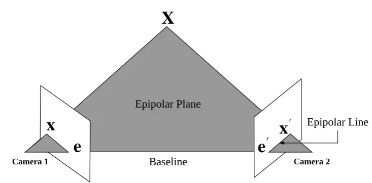
1.1 Illustration of the epipolar geometry. The optical centres of the two cameras and the 3D pointXdetermines the epipolar plane. Epipolese,e0 are defined as the intersection points of the baseline with each image plane. The epipolar plane and an image plane intersects at an epipolar line. . . 6

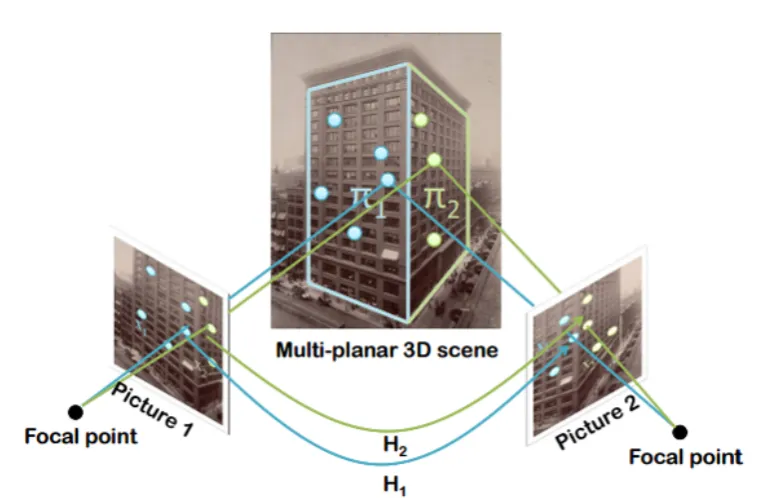
1.2 Illustration of a hompgrahy that associates the projections of a point on a planar structure. The raw image is from (Szpak et al. [2014]). . . 7

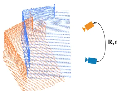
1.3 Illustration of point cloud registration problem. The point cloud is from (Sanchez et al. [2017]). The 3D camera and its observation are associated by using the same color. . . 9

1.4 Existing works that estimate the motion (rotation) of a camera by taking ad-vantage of the Manhattan World assumption. . . 10

1.5 Illustration of the 3D-2D registration problem. The goal is to estimate the relative pose of frame F_k+1 (with 2D information) w.r.t frame Fk (with 3D information). . . 10

1.6 Examples that use boundaries, edges and semi-dense regions around them. . . . 11

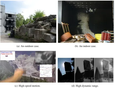
1.7 Illustration of challenging scenarios for classical vision based navigation. Im-ages are fromhttp://rpg.ifi.uzh.ch/gallery.html. . . 12 1.8 Illustration of an event camera and its working mechanism. Unlike standard

RGB cameras that capture the scene at a fixed frame rate, the event camera only reports “events” — intensity changes. The images are from (Rebecq et al. [2017b]). . . 14

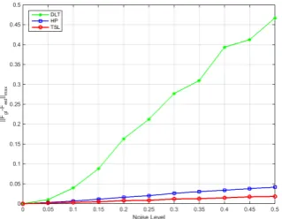
2.1 Figure (a) shows the configuration of the experiment. The accuracy of the fundamental matrix estimation is shown in Fig (b) with the max norm as the assessing criterion. Figures (c) (d) separately depict rotation and translation error of DLT, HP, TSL. . . 24

2.2 Grouped point features which are used for estimating the homographies are shown in Fig (a) and (b). Epipolar lines obtained by DLT(yellow), HP(green), TSL(blue) and groundtruth (red) are shown in Fig (c). . . 25

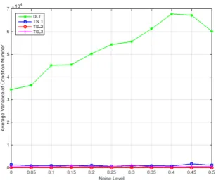
2.3 The average condition number under each noise level is shown in Figure (a). TSL1, TSL2 and TSL3 are the three sub least squares problems of TSL. Figure (b) shows the corresponding average variance of the condition number. . . 25

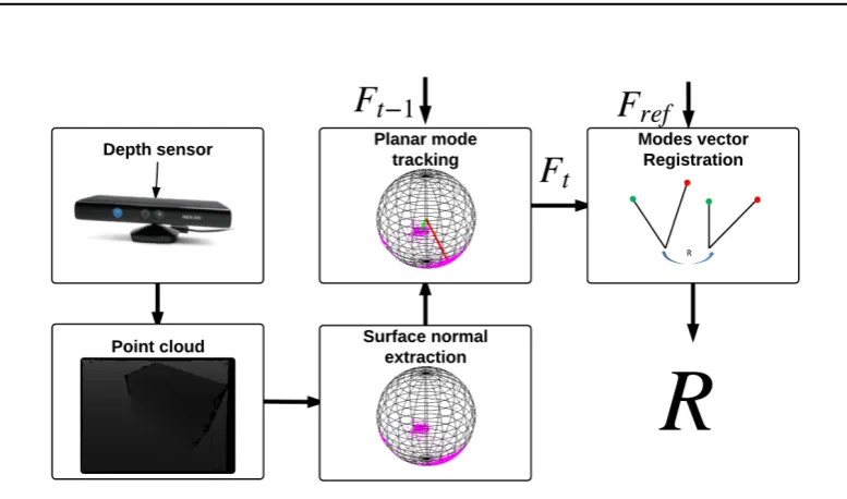
3.1 Overview of the proposed 3D rotation estimation algorithm for depth cameras in piece-wise planar environments. . . 28

(16)

xvi LIST OF FIGURES

3.2 Illustration of the geometry of the problem. Three modes exist in both the reference view (left) and the current view (right). The chordal distancedi be-tween each corresponding pair of modes is indicated with a black line segment. The relative rotation from the reference view to the current view is the solution that minimizes the sum of the chordal distances (in a general sense of`₁-norm regression). . . 32 3.3 Initialial mode seeking. The first figure shows the pattern that defines the

start-ing coordinates for the shift clusterstart-ing. The second figure shows a mean-shift in a tangential plane starting from a given coordinate. The histogram-based non-maximum suppression is shown in the third figure. It splits off mode centres by picking one mode and creating a histogram of rotation dis-tances with respect to all other modes. The final result after non-maximum suppression is shown in the last figure. Four planar modes are found and high-lighted with different colors. . . 33 3.4 Robustness of the rotation estimation. (a) (b) and (c) compare the performance

of the least-squares and the`₁-norm regression based methods for the case of 2, 3 and 4 modes, respectively. Note that in (a), the red line and the green line coincide with each other. The horizontal axes of (a), (b), and (c) denote the standard deviation of the noise that is imposed on the "badly tracked mode". (d) demonstrates the outlier resilience of the two methods for an increasing outlier fraction (10 modes in total). All the results (rotation error under each noise level and outlier number) are the average of 1000 trials with combination of arbitrary bundle structure and groundtruth rotation. . . 36 3.5 Performance evaluation on the synthetic dataset “Pyramid”. (a) shows the

syn-thetic scene which contains a ground plane and the four faces of a pyramid. The rotation estimation error is shown in (b). The estimated roll, pitch, and yaw angles are shown in (c). . . 37 3.6 The rotation estimation performance of the proposed algorithm without and

with the mode memory scheme. An obvious step-like curve in the top fig-ure again demonstrates the piece-wise drift-free behavior. The long-term drift compensation is shown in the bottom figure, where the blue dashed lines de-note the time instants when planar modes are revisited and the accumulated rotational drift gets compensated. . . 37 3.7 Illustration of the proposed algorithm running on a set of real sequences. Note

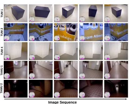
that images shown here are just to illustrate the scenes but are not used in the proposed algorithm. A unit sphere in the bottom-left corner of each image illustrates the planar mode bundle. Corresponding planes in each image of each sequence are denoted with the same color (e.g. the ground plane is always shown in red). We do not show results of TUM 3 because it has a similar scene as TUM 4. We also don’t show images for the ETH 1 dataset because it provides only point clouds. . . 39

(17)

LIST OF FIGURES xvii

4.2 Illustration of our cascaded manifold-constrained mean-shift implementation. We first compute updatessj for each mode onS2, which brings us from the black to the blue modes. The blue modes however do no longer represent a point on the underlying manifoldSO(3). We find the nearest rotation through a projection onto the manifold (green arrow), thus returning the red modes which are closest and at the same time fulfill the orthogonality constraint. . . . 47

4.3 The mechanism of the initial Manhattan frame seeking. The first figure shows the start from a random rotation. Each dominant direction is refined by per-forming a mean-shift iteration on the tangential space. The second figure shows the redundant result obtained by tracking 100 times from random starts. The redundancy of the estimated rotation matricesRis removed by first con-verting all theRto canonical form followed by a histogram-based non-maximum suppression. The final result is shown in the fourth figure. For the sake of clear visualization, the illustrated example contains a significant part of uniformly distributed noisy normal vectors. Note that the proposed seeking strategy is even able to find multiple MFs in the environment, and thus come up with a mixture of Manhattan frames. . . 48

4.4 The left figure shows an example of discretly sampled distribution truncated on the left and right sides (see red dashed lines). The right figure shows the convergence performance. After the truncation, the minimization problem has only one local minimum with a reasonably large convergence basin. . . 50

4.5 Robust MF seeking performance in several challenging cases. (a): Seeking the dominant MF when an additional mode/slanted plane exists. (b): Seeking the dominant MF in the case where only two modes can be observed. (c): The success rate of MF seeking under different levels of noise. . . 52

4.6 Simulation to demonstrate the benefit of performing the distribution alignment in the MF. . . 53

4.7 Evaluation of our method on the TUM datasetcabinetand comparison to two alternative odometry solutions (FastICP and DVO). Our method (red curve) works at 50 Hz on a CPU for VGA resolution depth images. It outperforms both DVO(blue curve, 30 Hz) and FastICP(cyan curve, 1 Hz) in terms of drift in rotation and translation. More detailed results can be found in Table 4.1 . . . 56

5.1 Image gradients are calculated in both horizontal and vertical direction at each pixel location. The euclidean norm of each gradient vector is calculated and illustrated in (a) (brighter means bigger while darker means smaller). Canny-edges are obtained by thresholding gradient norms followed by non-maximum suppression. By accessing the depth information of the edge pixels, a 3D edge map (b) is created, in which warm colors mean close points while cold colors represent faraway points. . . 61

(18)

xviii LIST OF FIGURES

5.3 Illustration of the point-to-tangent distance. The projected distanceris finally calculated by projectingvronto the direction of the local gradientg. . . 65 5.4 (a) Orientation bins chosen for the discretisation of the gradient vector

incli-nation (8 bins of 45◦ width). (b) Example oriented distance fields for edges extracted from an image of a football. Distinct edge segments are associated to only one of the 8 distance fields depending on the local gradient inclination and the corresponding bin. . . 67

5.5 Adaptively Sampled Nearest Neighbour Fields. In practice, the concatenated result is just an n×m matrix where the connected blue and green regions simply contain identical elements. . . 69

5.6 Sensor model is obtained by fitting the histogram with different probabilistic distributions. . . 71

5.7 Flowchart of the Canny-VO system. Each independent thread is bordered by a dashed line. CE refers to the Canny edge and DT is the abbreviation of distance transformation, which could be one of EDF, ANNF and ONNF. . . 72

5.8 Analysis of registration bias in case of only partially observed data. . . 74

5.9 Semi-dense reconstruction of two sequences from the TUM RGB-D bench-mark datasets. . . 75

5.10 Semi-dense reconstruction of the ICL_NUIMliving roomsequencekt2. . . 78

5.11 The schematic trajectory of the sensor when collecting the sequence is illus-trated in (a). The sequence starts from the position highlighted with a green dot. Structures such as window glass, plants, dark corridor caused by incon-sistent illumination that make the sequence challenging are shown in (b). . . 82

5.12 Evaluation on our own indoor sequence. The figures show different perspec-tives of the result obtained with and without loop closure enabled. . . 84

5.13 Close-up perspectives during the exploration of level 3 of the ANU Research School of Engineering. . . 84

5.14 Efficiency analysis on EDF, ANNF and ONNF based tracker. . . 85

6.1 Left: output of an event camera when viewing a rotating dot. Right: Time-surface map (6.1) at a timet, T(x,t), which essentially measures how far in time (with respect to t) the last event spiked at each pixel x = (u,v)T. The brighter the color, the more recently the event was generated. . . 90

6.2 Illustration of the geometry of the proposed problem and solution. The refer-ence view (RV) is on the left, in which an event with coordinates xis back-projected into 3D space with a hypothetical inverse depthρ. The optimal

in-verse depthρ?, lying inside the search interval[ρmin,ρmax], corresponds to the

(19)

LIST OF FIGURES xix

6.3 Verification of the proposed objective function. A randomly selected event in the reference view (RV) is marked by a red circle in (a). The overall energy is visualized in (b), with a red curve obtained by averaging the cost of all valid neighbouring observations (indicated by curves with random colors). The vertical dashed line (black) indicates the groundtruth inverse depth. The time-surface map of the left and the right event cameras at one of the observation times are shown in (c) and (d), respectively, where the patches for measuring the temporal residual are marked by red rectangles. . . 93 6.4 Distribution of the temporal residuals and Gaussian fitN(µ,σ2). . . 95

6.5 Illustration of the fusion strategy. All stereo observations(Ts

left,Trights )are

de-noted by hollow circles and listed in chronological order. Neighbouring RVs are fused into a chosen RV (e.g., RV3). Using the fusion from RV5 toRV3

as an example, the fusion rules are illustrated in the dashed square, in which a part of the image plane is visualized. The blue dots are the reprojections of 3D points inRV5on the image plane ofRV3. Gray dots represent unassigned

pixels which will be assigned by blue dots within one pixel away. Pixels that have been assigned,e.g. the green ones (compatible with the blue ones) will be fused. Pixels that are not compatible (in red) will either remain or be replaced, depending on which distribution has the smaller uncertainty. . . 96 6.6 Left, (a) and (b): the stereo event-camera rig used in our experiment, consisting

of two synchronized DAVIS (Brandli et al. [2014]) devices. Right, (c) and (d): rectified event maps at one time observation. . . 97 6.7 Results of the proposed method on several datasets. Images on the first

col-umn are raw intensity frames (not rectified nor lens-distortion corrected). The second column shows the events (undistorted and rectified) in the left event camera of a reference view (RV). Semi-dense depth maps (after fusion with several neighbouring RVs) are given in the third column, colored according to depth, from red (close) to blue (far). The fourth column visualizes the 3D point cloud of each sequence at a chosen perspective. No post-processing, such as regularization through median filtering (Rebecq et al. [2017a]), was performed. 100 6.8 Illustration of how the fusion strategy increasingly improves the density of the

reconstruction while reducing depth uncertainty. The first column shows the uncertainty mapsσρbefore the fusion. The second to the fourth columns report the uncertainty maps after fusing with 4, 8 and 16 neighbouring estimations, respectively. . . 101

(20)

(21)

List of Tables

2.1 Algorithm Complexity Comparison . . . 24

3.1 Performance comparison on several indoor datasets. . . 39

4.1 Performance comparison on several indoor dataset. . . 55

5.1 Comparison on the properties of different distance transformations . . . 70

5.2 Robust weight functions and their parameters fitted on each sub dataset . . . . 71

5.3 Relative Pose RMSE(R:deg/s,t:m/s) of TUM datasets . . . 76

5.4 Absolute Trajectory RMSE(m) of TUM datasets . . . 77

5.5 Relative pose RMSER:deg/s,t:m/s of ICL_NUIM . . . 79

5.6 Absolute Trajectory RMSE (m) of ICL_NUIM . . . 80

6.1 Quantitative evaluation on sequences with groundtruth depth. . . 98

(22)

(23)

Chapter1

Introduction and Contributions

Where am I? Who am I? How did I come to be here?

What is this thing called the world ...

Søren Kierkegaard, Danish philosopher.

As one of the hypotheses that may explain the burst of apparently rapid evolution in the lower Cambrian, the "Light Switch" theory of Parker [2016] believes that the evolution of eyes started an arms race that accelerated evolution. The rationale behind this hypothesis is that vision adds context of a scene, which enables creatures to more easily recognize food, a potential mate, or a predator. This is definitely an evolutionary advantage. Now, sighted crea-tures cover millions of species, from a part of invertebrates, such as some insects, to almost all vertebrates, including humans. From some molecularly similar chemoreceptor cells to pho-toreceptor cells, the eye experiences a long history of evolution to become a dedicated organ (Nilsson [1996]). These special cells are very sensitive to light, more accurately photons. The signals of those photons are transmitted to the brain, where they are decoded as colors and shapes. Modern cameras work in the similar principle as our eyes do, whereas imaging chips (e.g. semiconductor charge-coupled devices (CCD) or active pixel sensors in complementary metal–oxide–semiconductor (CMOS)) play the role of photoreceptor cells. With these artifi-cial eyes, researchers expect to endow robots the ability to perceive the world visually as we humans do. The missing part right here is the “algorithm” in robots’ brains to process the data. When stepping into an unknown environment, like humans, the first priority of a robot is to be aware of where it is and what the surrounding environment is like. Vision based ego-motion estimation, coined as Visual Odometry (VO) by Nistér et al. [2004], has been an active field of research for more than three decades. It has wide application domains including augmented reality (AR) and autonomous driving,etc.Specifically, VO plays an essential role in the field of robotic control and navigation when no external reference signal is available. Examples are given by rovers operating on Mars (Moravec [1980]; Lacroix et al. [1999]), autonomous underwater vehicles (AUVs) carrying out exploration under the ocean (Corke et al. [2007]; da Costa Botelho et al. [2009]) and unmanned aerial vehicles (UAVs) patrolling in a GPS-denied environment, such as an indoor scene, a forest or an urban canyon (Courbon et al. [2009]; Tomic et al. [2012]; Forster et al. [2013]; Langelaan and Rock [2005]), etc. All of above systems need an alternative navigation modality which helps the robots to know their

(24)

2 Introduction and Contributions

own status of motion with respect to surrounding environments.

1 .

1 History of VO

The term VO was first used by Srinivasan et al. [1997] to define motion orientation of honey bees. This term has become popular in the field of computer vision and robotics since the paperVisual Odometry(Nistér et al. [2004]) was published. However, in fact the first known work implementing this idea is a stereo VO system by Moravec [1980] for NASA’s Mars rover in 1980. The goal of the project is to give an alternative to wheel odometry which is always affected by slippage in uneven terrains. In the following two decades, the research on VO was led by NASA/JPL in preparation for the 2004 Mars mission (Matthies and Shafer [1987]; Matthies [1989]; Lacroix et al. [1999]; Olson et al. [2000]).

Stereo cameras are the most popular choice in the early solutions (Matthies and Shafer [1987]; Matthies [1989]; Lacroix et al. [1999]; Olson et al. [2000, 2003]; Cheng et al. [2005]; Milella and Siegwart [2006]; Howard [2008]). The reason is that stereo systems can recover 3D information without a prior of motion, which turns the estimation of the relative pose into a process of solving a straightforward 3D-to-3D point registration problem. Different motion estimation schemes are introduced by Nistér et al. [2004] and Comport et al. [2007]. Nistér et al. [2004] performed a 3D-to-2D point registration while Comport et al. [2007] relied on the quadrifocal tensor, which allowed motion estimation to be computed from 2D-to-2D image matches without having to triangulate 3D points.

An alternative to stereo based solutions is to use a single camera. The reason of interest in the monocular case is three-fold. First, stereo systems need to be calibrated intrinsically and extrinsically, which makes them more complicated compared to monocular systems. Second, multiple cameras will lead to additional energy consumption, which may not be available to some small mobile platforms. Last but not the least, a stereo system is known as to degenerate to the monocular case when the distance from the cameras to the scene becomes much bigger than the length of the baseline.

Some of existing works are worth special mentioning because they either created standards and inspired following works or still represent the state of the art.

1.1.1 Probabilistic Filter based Monocular SLAM

(25)

§1.1 History of VO 3

1.1.2 Nister’s VO

Nister et al.made several contributions to the field of VO. First, they presented an efficient five-point algorithm (Nistér [2004]) which would not degenerate in the case of coplanarity as the normalized eight-point algorithm (Hartley [1997]) does. Second, they provided a 3D-to-2D formulation of VO (Nistér et al. [2004]), which performs 3D reconstruction and camera pose estimation in an alternated fashion. More importantly, they concluded that the 3D-to-2D scheme is more accurate compared to either the 2D-to-2D or the 3D-to-3D scheme.

1.1.3 Parallel Tracking and Mapping (PTAM)

The standard of the front-end for modern SLAM systems is set by a work from the commu-nity of AR. Parallel tracking and mapping, also known as PTAM, was proposed by Klein and Murray [2007]. PTAM is a feature based method and follows the 3D-to-2D formulation de-scribed in (Nistér et al. [2004]). Its original design consists of decoupling the mapping from the tracking. This enables keyframe based bundle adjustment (BA) (Triggs et al. [1999]) that optimizes over many more points than the filter based method. Moreover, PTAM does not need to maintain an estimate of a dense covariance matrix as Mono-SLAM does, therefore much faster.

1.1.4 State of the Art

Based on the schemes of previous works, state-of-the-art systems keep making improvement from perspectives of both theory and system engineering. Based on the different information used for motion estimation, they could be clustered into four categories: feature based methods, direct methods, hybrid methods, and methods based on 3D point set registration.

• Feature based methods:

The front-end of ORB-SLAM (Mur-Artal et al. [2015] is a feature-based method and is quite similar to PTAM. It achieves better performance compared to PTAM by 1) extend-ing an additional thread for loop closextend-ing which guarantees globally consistent localiza-tion and mapping; 2) automatically initializing the map via selecting a model between the Homography and the Fundamental matrix, while PTAM requires manual operation to finish the initialization; 3) utilizing ORB features (Rublee et al. [2011]) instead of image patches used in PTAM which improves matching accuracy under scale and orientation changes; 4) multi-scale mapping which consists of a local graph for pose refinement, a co-visibility graph for local bundle adjustment, and an essential graph for global bundle adjustment after a loop closing is detected and verified.

• Direct methods:

(26)

However, processing every pixel over all image sequences is very computationally ex-pensive which leads to dependency on GPU hardwares. The appearance of low cost RGB-D cameras eliminates the estimation of depth maps, which makes it applicable for running fully dense methods on CPU in real time. Kerl et al. proposed a dense visual odometry (DVO) (Kerl et al. [2013a]). The relative pose between two frames is estimated by solving a 3D-2D registration problem. A probabilistic formulation is given for improving the robustness in the presence of outliers and sensor noises. More recently, Engelet al.proposed a semi-dense visual odometry (SDVO) using a monoc-ular camera (Engel et al. [2013]). SDVO only uses pixels that are along the boundary of structures. Therefore, it is able to run in real-time on a CPU. SDVO utilizes the same tracking method as DVO does. The contribution of SDVO is the probabilistic fusion based mapping, in which measurement uncertainties originating from both geo-metric and photogeo-metric cues are effectively modelled. More recently, Engel et al. [2017] present the direct sparse odometry (DSO), which applies direct method on a number of sparse points. These sparse points are sampled across image areas with sufficient inten-sity gradient. To deal with imperfect brightness constancy, Engel et al. [2017] propose a photometric calibration pipeline, which recovers the irradiance images and therefore increases the tracking accuracy.

• Hybrid methods:

Direct methods are known to be sensitive to inconsistent illumination, while feature-based approaches fail when not enough textures appear. Hybrid methods have claimed a better performance in these challenging cases. For example, Scaramuzza and Siegwart [2008] used the image appearance to estimate the rotation of the car and features from the ground plane to estimate the translation and the absolute scale. Forster et al. [2014] used the photometric information around sparse features, which leads to precise, robust and amazingly fast performance (400 fps on a laptop).

• 3D point registration based methods:

(27)

§1.2 Motivation and Objectives — Exploiting Structural Regularities and Beyond 5

1 .

2 Motivation and Objectives — Exploiting Structural

Regu-larities and Beyond

By looking at the history of VO, we see that a lot of efforts have been made in order to achieve efficient pose estimation while keeping the global drift as small as possible. Among the mas-sive body of existing work, few of them focus on improving the tracking performance via taking advantage of the structural prior hidden in structural regularities of man-made environ-ments.

As a frequently occuring geometric regularity in man-made environments, planar struc-tures provide a strong geometric constraint on ego-motion estimation. In the 2D relative pose problem, the co-planarity of points leads to a compact expression of motion and structure — the homography. It is believed that a prior on the structure would benefit the motion estima-tion and vice versa (Szeliski and Torr [1998]), thus, the estimaestima-tion of the fundamental matrix would ideally benefit from using homographies as input. When 3D information is available, the piece-wise planar environment enables us to create alternative solutions to ICP, which is computationally expensive and suffers from local minimums. We show that the surface nor-mal vectors of those planes can be used to efficiently estimate the relative rotation between different perspectives. Moreover, if the environment consists of three dominant planes that are orthogonal to each other, namely a Manhattan World (MW), the rotation estimation is glob-ally drift-free while each degree of translational freedom could be further solved in parallel. A more general structure regularity is the contours/edges. They typically correspond to pixels with strong intensity gradient in images. Pose estimation based on these pixels are less affected when the photometric consistency assumption does not strictly hold. We can see that both the efficiency and the accuracy benefits from exploiting structural regularities in this research. However, when application scenarios bring in challenging conditions such as high-speed mo-tion, high dynamic range (HDR) that are beyond what normal sensors (standard RGB/RGB-D cameras) can handle, existing solutions are no longer applicable. Accordingly, it is imperative to investigate recently emerging sensors and to develop novel algorithms that fit their distinct characteristics.

1.2.1 2D Geometrically Constrained Relative Pose Estimation: Points on

Planes

The epipolar geometry of two perspective images, illustrated by Fig. 1.1, demonstrates that a 3D pointXobserved in one image must lie (when no occlusion exists) on the epipolar line in the other image. This constraint can be described by a singular3×3matrix. When the camera is calibrated, the matrix is known as the essential matrix E. For uncalibrated systems, it is known as the fundamental matrixF. The estimation of the fundamental matrix is a classical and thoroughly studied topic which plays an essential role in many applications involving multiple-view geometry.

The most popular method for estimating the fundamental matrix is to solve Eg. 1.1 given sparse correspondences between local invariant keypoints, for instance SIFT features (Lowe [2004]).

(28)

Epipolar Plane

Baseline

Camer a 1 Camer a 2

[image:28.595.94.461.102.283.2]

Epipolar Line

Figure 1.1: Illustration of the epipolar geometry. The optical centres of the two cameras and the 3D point Xdetermines the epipolar plane. Epipoles e, e0 are defined as the intersection points of the baseline with each image plane. The epipolar plane and an image plane intersects

at an epipolar line.

Using the direct linear transform (DLT), Eq 1.1 is transformed into a linear equation system

Af=



 

x0₁x1 x01y1 x01 y10x1 y01y1 y01 x1 y1 1

..

. ... ... ... ... ... ... ... ...

x0_nxn x0nyn x0n yn0xn y0nyn y0n xn yn 1





f=0, (1.2)

where (xi,yi) ↔ (x0i,y0i),i = 1· · ·n, denotes the feature correspondences, and f consists of all entries of the fundamental matrixF. Seven points constitute the minimal configuration because the fundamental matrix has 7 degrees of freedom (DoF). Compared to the eight-point algorithm, the seven point algorithm needs an additional step to calculate the linear combi-nation factor of the obtained two-dimensional null-space. While seven point correspondences represent the minimum for estimating the fundamental matrix (Stewart [1999]), the eight-point algorithm (Longuet-Higgins [1987]) is the most widely used method because of its linear na-ture and thus simplicity to implement. However, it was only after Hartley published his seminal work (Hartley [1997]) on using data normalization that the eight-point algorithm became truly useful in practice.

When a point is on a plane, its projections on two images can be associated by not only a fundamental matrix, but also a homography. The association is denoted by Eq. 1.3 and the geometry is illustrated in Fig. 1.2.

x0 =Hx (1.3)

(29)

[image:29.595.125.515.103.352.2]

Figure 1.2: Illustration of a hompgrahy that associates the projections of a point on a planar structure. The raw image is from (Szpak et al. [2014]).

(30)

1.2.2 Tracking a 3D Sensor in Piece-wise Planar Environments and

Man-hattan Worlds

3D sensors typically refer to devices that are able to obtain the 3D information of a scene, especially those that provides dense 3D measurements, such as Velodyne LiDARs, Microsoft Kinects and so on. The problem of tracking a 3D sensor is typically formulated as a point cloud registration problem, shown as Fig. 1.3. A 3D point cloud can be denoted as P = pi,i=1, ...,M, wherepirepresents the coordinate of a 3D point, and Mis the number of 3D points in the point cloud. Assume a 3D camera captures a scene at two different perspectives and generates two point cloudsP,Q. Since the coordinate of the point cloud is described in the camera coordinate system, to estimate the relative pose between two different perspectives is equivalent to rigidly registering the two point clouds. The point cloud registration problem is generally written as

R,t=arg min

R,t

Φ(G(P,R,t),Q), (1.4)

where(R,t) ∈ SE(3), function Gapplies rigid transformation (R,t) onP, andΦ(·,·) mea-sures the registration error in a certain metric. The most commonly used way to solve prob-lem 1.4 is the ICP algorithm (Besl and McKay [1992]), in which the registration error in 1.4 is defined as the sum of the squared closest-point distances,

R,t=arg min

R,t

M

∑

i=1

min

j=1,···,NkRpi+t−qjk

2_, _(1.5)

where pi,i = 1,· · · ,M andqj,j = 1,· · · ,N denote the 3D points in P and Q, respec-tively. The ICP algorithm performs registration through iterative minimization of the sum of the squared closest-point distances between spatial neighbours in two point sets.

In order to avoid the costly repetitive derivation of point-to-point correspondences, the community has also investigated the representation and alignment of point clouds using density distribution functions. The idea was proposed by Chui and Rangarajan [2000a] and Tsin and Kanade [2004], who represented point clouds as explicit Gaussian Mixture Models (GMM) or implicit Kernel Density Estimates (KDE), and then found the relative transformation (not necessarily Euclidean) by aligning those density distributions. Jian and Vemuri [2011] sum-marized the idea of using GMMs for finding the aligning transformation, and notably derived a closed-form expression for computing the L2 distance between two GMMs. Yet another alternative which avoids the establishment of point-to-point correspondences was given by Fitzgibbon [2003], who utilizes a distance transformation in order to efficiently and robustly compute the cost of an aligning transformation. The distance transformation itself, however, is again computationally intensive.

(31)

[image:31.595.125.517.100.392.2]

Figure 1.3: Illustration of point cloud registration problem. The point cloud is from (Sanchez et al. [2017]). The 3D camera and its observation are associated by using the same color.

successful application of local methods.

Planar structures in man-made environments can benefit both tracking and mapping per-formance when using exteroceptive sensors. Weingarten and Siegwart [2006] and Trevor et al. [2012] used planar-segment features extracted from 3D sensors. Both of them claimed that the planar segments can be used to improve the data association, which in turns benefits the whole localization and mapping process. Taguchi et al. [2013] combined point and plane features towards fast and accurate 3D registration. From exterior side to interior side, modern buildings frequently contain orthogonal structures in the surface arrangement. The property was coined asManhattan World(MW) in (Coughlan and Yuille [1999]), where they formulated vanishing point estimation from a single RGB image as a Bayesian inference problem. Košecká and Zhang [2002] presented a video compass using a similar idea. Tracking theManhattan Frame

(32)

estimation of the rotation of a camera through tracking theManhattan Frame. Few have shown how to perform a full 6-Dof motion estimation based on the Manhattan assumption.

(a) Coughlan and Yuille [1999]. (b) Košecká and Zhang [2002]. (c) Straub et al. [2015a].

Figure 1.4: Existing works that estimate the motion (rotation) of a camera by taking advantage of the Manhattan World assumption.

1.2.3 One Step Beyond: A More General Regularity — Edges

3D

2D

Figure 1.5: Illustration of the 3D-2D registration problem. The goal is to estimate the relative pose of frameF_k+1(with 2D information) w.r.t frameFk (with 3D information).

(33)

(a) Engel et al. [2013, 2014]. (b) Nurutdinova and Fitzgibbon [2015].

(c) Kuse and Shen [2016].

Figure 1.6: Examples that use boundaries, edges and semi-dense regions around them.

Nurutdinovaet al. presented a method which uses parametric curves as landmarks for motion estimation and BA (Nurutdinova and Fitzgibbon [2015]). In contrast, non-parametric methods are more popular. Engelet al. applied direct photometric registration to semi-dense regions defined as all neighbouring pixels of edges (Engel et al. [2013, 2014]). A more relevant work to this thesis is (Kuse and Shen [2016]), which presents a direct edge alignment approach for 6-DOF tracking. Non-parametric methods are always formulated as a 3D-2D registration problem, as illustrated by Fig. 1.5. When using photometric measurements (Newcombe et al. [2011b]; Engel et al. [2013, 2014]; Schoeps et al. [2014]), the objective function is written as,

R,t=arg min

R,t

∑

i

(I_k+1(W(xi,zi;R,t))−Ik(xi))2 (1.6)

whereI(·)returns the intensity of a given pixel coordinate,W(·)warps a pixel under its depth

ziand the optimized motion parametersR,t. The optimal motion leads to the global minimum of the objective function. When the residuals are measured in geometric distance (Kneip et al. [2015]; Kuse and Shen [2016]; Zhou et al. [2017]), the objective function is denoted as,

R,t=arg min

R,t

∑

i

D(W(xi,zi;R,t)) (1.7)

whereD(·)returns the distance to the closest point. The objective function is typically solved as an 3D-2D ICP problem, which needs to repeatedly search for the closest point for each warping pixel in each iteration. To accelerate the closest point searching,distance transform

(DT) is introduced by Felzenszwalb and Huttenlocher [2004]. A look-up table under a certain distance metric is created to avoid repeated searching.

(34)

big motion, a coarse-to-fine strategy is typically used (Kuse and Shen [2016]). Nurutdinova and Fitzgibbon [2015] overcame the partial occlusion problem by using parametric curves while increasing the dimension of unknowns. Furthermore, robust tracking requires to handle outliers and noises effectively. Most of the exiting pipelines just empirically choose robust weight function rather than looking into the real probabilistic characteristics of the sensor.

1.2.4 Beyond the Limits: Event-based VO

When applying VO/SLAM techniques in practical applications, more complicated and chal-lenging scenarios than what we see in the laboratory could emerge. An example is illustrated in Fig 1.7, in which a small UAV is performing a rescue task in a post-disaster environment. Fast operations are very much expected to save more lives. Therefore, image blur induced by high-speed motions must be handled. Besides, the drone may fly from indoor to outdoor, which can lead to severe illumination changes. In extreme cases, over/under-exposure can make that sys-tem sys-temporarily blind. Thus, an ideal sensor needs to be capable of dealing with high dynamic range (HDR) scenarios. Each of these challenging factors can easily fail existing VO/SLAM solutions developed for traditional visual sensors. Accordingly, it is imperative to investigate recently emerging sensors and to develop novel algorithms that fit their distinct characteristics.

(a) An outdoor case. (b) An indoor case.

[image:34.595.90.469.410.698.2]

(c) High-speed motion. (d) High dynamic range.

(35)

§1.3 Thesis Outline and Contributions 13

Event cameras, such as the Dynamic Vision Sensor (DVS) (Lichtsteiner et al. [2008]), are novel devices that output pixel-wise intensity changes (called “events”) asynchronously, at the time they occur. As opposed to standard cameras, they do not acquire an entire image frame at the same time, nor do they operate at a fixed frame rate. An illustration of the event camera’s working mechanism is given in Fig. 1.8. The output of an event camera is a 3D spatial-temporal signal, which is typically denoted as a tuple,

e={u,v,t,p}, (1.8)

whereu,vdenotes the event coordinate on the sensor plane, tgives the timestamp when the event occurs and ptells the sign of the intensity change. This asynchronous and differential principle of operation reduces power and bandwidth requirements drastically. Endowed with microsecond temporal resolution, event cameras are able to capture high-speed motions, which would typically cause severe motion blur with standard cameras. In addition, event cameras have a very high Dynamic Range (HDR) (e.g.140dBcompared to 60dBof most standard cam-eras), which allows them to be used under a broad range of illumination. Hence, event cameras open the door to tackle challenging scenarios that are inaccessible to standard cameras, such as high-speed and/or HDR tracking (Mueggler et al. [2014]; Lagorce et al. [2015]; Zhu et al. [2017]; Gallego et al. [2017]), control (Conradt et al. [2009]; Delbruck and Lang [2013]) and Simultaneous Localization and Mapping (SLAM) (Kim et al. [2016]; Rebecq et al. [2017c]; Rosinol Vidal et al. [2018]).

The main challenge in visual processing with event cameras is to devise specialized algo-rithms that can exploit the temporally asynchronous and spatially sparse nature of the image data produced by DVS cameras, hence unlocking their full potential, whereas existing com-puter vision algorithms designed for conventional cameras do not directly apply in general. Some preliminary works on DVS addressed this issue by combining event cameras with other sensors, such as standard cameras (Censi and Scaramuzza [2014]; Kueng et al. [2016]) or depth sensors (Censi and Scaramuzza [2014]; Weikersdorfer et al. [2014]), in order to simplify the task at hand. Although this approach obtained certain success, the true potential of an event camera has not been fully exploited since parts of such combined systems are limited by the lower dynamic range devices.

1 .

3 Thesis Outline and Contributions

(36)

at-14 Introduction and Contributions

(a) Event camera. (b) Working mechanism.

Figure 1.8: Illustration of an event camera and its working mechanism. Unlike standard RGB cameras that capture the scene at a fixed frame rate, the event camera only reports “events” —

intensity changes. The images are from (Rebecq et al. [2017b]).

tractive hallucinated points based method. The algorithm is theoretically justified and verified by experiments on both synthetic and real data.

In Chapter. 3, an efficient 3D rotation estimation algorithm for depth cameras in piece-wise planar environments is presented. It shows that by using surface normal vectors as an input, planar modes in the corresponding density distribution function can be discovered and continu-ously tracked using efficient non-parametric estimation techniques. The relative rotation from the reference view to the current view can be estimated by registering entire bundles of pla-nar modes. Robustness of the bundle registration process is achieved by performing a general `₁-norm regression instead of simply solving a least-squares problem. Piece-wise drift-free performance is achieved as long as no bundle updates happen.

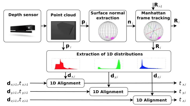
In Chapter. 4, we reply on the results of Chapter. 3 and make the further assumption about the environment that three mutually orthogonal planes exit. A highly efficient motion esti-mation framework is presented for 3D sensors such as the Microsoft Kinect v.2, based on alignment of density distribution functions. Absolute rotation is estimated by exploiting the properties of Manhattan Worlds, thus resulting in a manifold-constrained multi-mode tracking scheme. The individual translational degrees of freedom is efficiently estimated through 1D kernel density estimates. A real-time implementation is given, which is able to process dense depth images with VGA resolution at more than 50Hz on a CPU.

(37)

§1.3 Thesis Outline and Contributions 15

choice from various robust M-Estimators. The proposed method outperforms state-of-the-art edge-alignment based method in terms of accuracy, efficiency and robustness.

In Chapter 6, to deal with challenging scenarios that are beyond what standard RGB/RGB-D cameras can handle, we investigate a recently emerging sensor — the event camera — and focus on the problem of 3D reconstruction from data captured by a stereo event-camera rig moving in a static scene, such as in the context of stereo Simultaneous Localization and Mapping. The proposed method consists of the optimization of an energy function designed to exploit small-baseline spatio-temporal consistency of events triggered across both stereo image planes. To improve the density of the reconstruction and to reduce the uncertainty of the estimation, a probabilistic depth-fusion strategy is also developed. The resulting method has no special requirements on either the motion of the stereo event-camera rig or on prior knowledge about the scene. Experiments demonstrate the proposed method can deal with both texture-rich scenes as well as sparse scenes, outperforming state-of-the-art stereo methods based on event data image representations.

1.3.1 Publication

The thesis is mainly based on the following publications during my PhD:

– Zhou et al. [2015] Y. Zhou, L. Kneip and H. Li, "A Revisit of Methods for Determin-ing the Fundamental Matrix with Planes," 2015 International Conference on Digital Image Computing: Techniques and Applications (DICTA), Adelaide, SA, 2015, pp. 1-7.

– Kneip et al. [2015] L. Kneip, Y. Zhou and H. Li. "SDICP: Semi-Dense Tracking based on Iterative Closest Points". In Proceedings of the British Machine Vision Conference (BMVC), pages 100.1-100.12. BMVA Press, September 2015.

– Zhou et al. [2016a] Y. Zhou, L. Kneip and H. Li, "Real-time rotation estimation for dense depth sensors in piece-wise planar environments," 2016 IEEE/RSJ Interna-tional Conference on Intelligent Robots and Systems (IROS), Daejeon, 2016, pp. 2271-2278.

– Zhou et al. [2016b] Y. Zhou, L. Kneip, C. Rodriguez, and H. Li. "Divide and conquer: Efficient density-based tracking of 3D sensors in Manhattan worlds." In Asian Con-ference on Computer Vision (ACCV), pp. 3-19. Springer, Cham, 2016.

– Zhou et al. [2017] Y. Zhou, L. Kneip and H. Li, "Semi-dense visual odometry for RGB-D cameras using approximate nearest neighbour fields," 2017 IEEE International Conference on Robotics and Automation (ICRA), Singapore, 2017, pp. 6261-6268.

– Zhou et al. [2018b] Y. Zhou, H. Li, L. Kneip, "Canny-VO: Visual Odometry with RGB-D Cameras based on Geometric 3D-2D Edge Alignment," accepted by IEEE T-RO (published as Early Access by far).

(38)

(39)

Chapter2

2D Geometrically Constrained

Relative Pose Estimation: Points on

Planes

In this chapter, we look into the problem of relative pose estimation in piece-wise planar en-vironments. More specifically, we focus on answering a classical visual geometry question – how to determine the fundamental matrix from a collection of inter-frame homographies (more than two). The compatibility relationship between the fundamental matrix and any of the ide-ally consistent homographies can be used to compute the fundamental matrix. Using the direct linear transformation (DLT), the compatibility equation can be translated into a least squares problem and easily solved via SVD decomposition. However, this solution is extremely sus-ceptible to noise and motion inconsistencies, hence rarely used. Inspired by the normalized eight-point algorithm, we show that a relatively simple but non-trivial two-step normalization for the input homographies achieves the desired effect, and the results are at least comparable to the less attractive hallucinated points method. The algorithm is theoretically justified and verified by experiments on both synthetic and real data.

2 .

1 Related Work — Three Classical Methods

Szeliski and Torr discussed three methods that can be used for the estimation of the fundamen-tal matrix given several(_>2)homographies in (Szeliski and Torr [1998]), which are reviewed in the following.

• Hallucinating additional correspondences:

Hallucinated points refer to augmented sample points on planes. Theses points are also called virtual control points. Hallucinated correspondences are generated by first creat-ing several virtual 2D pointsxon image one which are assumed to be the projection of virtual points on the plane. Their corresponding pointsx0are then found by applying the corresponding homography to pointsx. Then the fundamental matrixFis computed by applying normalized 8-point algorithm on the obtained hallucinated correspondences.

• Direct linear method:

(40)

18 2D Geometrically Constrained Relative Pose Estimation: Points on Planes

The implicit compatibility relationship between inter-frame homographies and the fun-damental matrix can be directly used for computing the funfun-damental matrix. The com-patibility equationFTH+HTF =0gives six constraints (Luong and Faugeras [1993]) (for which only 5 are linearly independent). Therefore, at least 2 homographies are needed for computing the fundamental matrix. The question can be translated to a least squares problem by DLT and can be easily solved by SVD decomposition. However, this straightforward method is unstable for inaccurate homographies, sometimes leading to completely meaningless results. The reason given by Szeliski and Torr is that using the compatibility equation directly corresponds to sampling homographies at locations where their predictive power is very weak. The samples are far from having the normal distribution required for total least squares to work reasonably well.

• Plane plus parallax:

Plane plus parallax techniques are always used to recover the depth (projective or Eu-clidean) of the scene. To compute the fundamental matrix, one of the homographies is chosen and used to warp all the feature points to the current frame. The epipolee0 is computed by minimizing the sum of the weighted distance between the epipole and lines passing through corresponding pointsxi andx0_i. Then the fundamental matrixFcan be computed byF = [e0]×H. This method cannot work well when points are evenly dis-tributed over several planes. The computation is also more complicated and expensive compared to the former two methods.

2 .

2 A Robust Two-Step Linear Solution

The compatibility equationFTH+HTF=0gives only 6 linear equations (Luong and Faugeras [1993]). In fact, as shown later, only 5 of them are independent. Therefore, at least 2 homo-graphies are needed to compute the fundamental matrix. Applying the DLT transformation to the compatibility equation leads to the least squares problem,

Af=      W1 W2 .. . Wn     

f=0, (2.1)

wheref = (f11,f21,f31,f12,f22,f32,f13,f23,f33)T denotes a vector obtained by rearranging

the entries of the fundamental matrix in a column vector. MatrixAis made up of several sub matricesWiof same dimension which is defined as,

Wi =

      

2hπ₁₁i 0 0 2h₂₁πi 0 0 2hπ₃₁i 0 0

hπi

12 h

π_i

11 0 h

π_i

22 h

π_i

21 0 h

π_i

32 h

π_i

31 0

hπ₁₃i 0 hπ₁₁i hπ₂₃i 0 hπ₂₁i hπ₃₃i 0 hπ₃₁i

0 2hπi

12 0 0 2h

π_i

22 0 0 2h

π_i

32 0

0 hπi

13 h

π_i

12 0 h

π_i

23 h

π_i

22 0 h

π_i

33 h

π_i

32

0 0 2h13 0 0 2hπ23i 0 0 2h

(41)

§2.2 A Robust Two-Step Linear Solution 19

The entries of the matrixWi originate from the homographyHi =





hπi

11 h

πi

12 h

πi 13

hπi

21 h

πi

22 h

πi 23

hπi

31 h πi 32 h πi 33  which

is induced by plane π_i. The least squares problem described in Eq. (2.1) is seriously

ill-conditioned, which means that even under a tiny perturbation of any entry of matrixA, the solu-tion quickly diverges from the groundtruth result. Thus, the matrixAshould be re-conditioned in order to stabilize its null space.

The presented method follows the idea of Hartley [1997] and introduces normalization in order to stabilize the result. However, it is not trivial to directly normalize the matrixAas it has been done in prior work for estimating the fundamental matrix or even the homography from point correspondences. The reason is two-fold. First, the normalization includes two parts, translation and scaling. The translation operation can only be performed by a linear transformation when the normalized object is described in the homogeneous form. Second, the normalization should be performed to data which have the same physical meaning.

The key to deal with the above two issues comes from the special structure of the matrix FTH. The compatibility equation requires thatFTHis a skew-symmetric matrix, and thus is of the form

FTH=





0 −a3 a2

a3 0 −a1

−a2 a1 0 

. (2.3)

The diagonal entries give three equations which describe an orthogonal relationship between corresponding column vectors of the fundamental matrix and a homography,

f_iThi =0,i=1, 2, 3. (2.4)

fi andhi denote theith column vector of the fundamental matrix F = f1 f2 f3

and the homographyH= h1 h2 h3

. The other three equations enforce the skew symmetric prop-erty. However, only two of them are independent. This makes sense because a homography has 8 degrees of freedom (DoF). For the uncalibrated case, the intrinsic matrix is unknown which removes three constraints. Thus, only five independent constraints can be obtained from one homography, three from the orthogonal relationship described in Eq. (2.4) and the other two from the skew-symmetric property.

Our two-step reconditioning method realizes the non-trivial normalization by fully using the special structure of matrixFTH. First, by utilizing the orthogonal relationship, we decom-pose the original least squares problemAf=0into three sub least squares problemsAifi =0, where matrixAi = hπ_i1 hπ_i 2 · · · hπ_in

T

andi = 1, 2, 3. Each column of the fundamen-tal matrix fi is estimated individually. The relative scale factor for each estimated solution fi can then be recovered by using the skew-symmetric property of matrixFTHin Eq. (2.3). With this formulation, every column of matrixAi has the same physical meaning. Besides, in order to perform the translation, the matrixAi should be extended by an additional column 13×1 = (1 1 1)T which leads toA˜i = [Ai|13×1]. Accordingly, the extended solution

vec-tor˜f_iis defined as˜f_i =

λ_i−1fi

0

, whereλdenotes the relative scale factor of the individually

(42)

20 2D Geometrically Constrained Relative Pose Estimation: Points on Planes

The mathematical proof is given after the whole algorithm is introduced.

The normalization is then performed by inserting a4×4linear transformation matrixQi and its inverse in betweenA˜iand˜fi, resulting in

˜

AiQiQ−i 1˜fi =Aˆiˆfi =0, (2.5) where Aˆi = A˜iQi and ˆfi = Qi−1˜fi. The linear transformation Qi includes a translation and a scaling. We regard each hπ_ij as a 3D point. Following the idea of Hartley [1997], the coordinates are translated such that the centroid c of the set of all such points becomes the origin. The coordinates are then scaled by applying an isotropic scaling factor sto all three coordinates of each point. Finally, we choose to scale the coordinates such that the average distance of a pointhπ_i j from the origin is equal to√3. The linear transformationQiand scaling related variables are defined as,

Qi =



  

s 0 0 0

0 s 0 0

0 0 s 0

−c1s −c2s −c3s 1 

  

, (2.6)

c= c1 c2 c3 T

= ∑ m j=1h

πj

i

m , (2.7)

s= √

3 ¯

d , ¯d=

∑m j=1kh

πj

i −ckF

m . (2.8)

The solution of the three sub least squares problemsAˆiˆfi = 0can be easily obtained via SVD. Then˜fi =Qiˆfi. The only remaining task is to find the scale factorsλi.

The skew-symmetric property of matrixFTHcan be translated into another least squares problemAλλ=0via DLT, whereλ= λ1 λ2 λ3

T

andAλis given by

Aλ =

          ˜fT 1,1:3h π₁

2 ˜fT2,1:3h

π₁

1 0

˜fT

1,1:3h

π₁

3 0 ˜f3,1:3T h

π₁

1

0 ˜fT

2,1:3h

π₁

3 ˜f3,1:3T h

π₁

2

..

. ... ...

˜fT

1,1:3h2πm ˜fT2,1:3hπ1m 0

˜fT

1,1:3h3πm 0 ˜fT3,1:3hπ1m

0 ˜fT

2,1:3hπ3m ˜fT3,1:3hπ2m

          . (2.9)

˜fi,1:3inAλis defined as the first three rows of vector˜fi.h

πj

i is defined the same as before. The full two-step linear method (TSL) is described in Algorithm 1.

It should be noted that in order to apply the normalization, the original least squares prob-lem is modified. However, we will see in the following that solving the modified probprob-lem

˜

Ai˜fi = 0is equivalent to solving the original problem Aifi = 0. Therefore, two questions need to be answered in order to prove this claim:

1. After extending the matrixAi by an additional column13×1 = (1 1 1)T, what is the