Large Scale Classification Based on Combination of
Parallel SVM and Interpolative MDS
Sun Zhanquan
1, Geoffrey Fox
2(1 Key Laboratory for Computer Network of Shandong Province, Shandong Computer Science Center, Jinan, Shandong, 250014, China
2 School of Informatics and Computing, Pervasive Technology Institute, Indiana University Bloomington, Bloomington, Indiana, 47408, USA)
[email protected], [email protected]
Abstract: With the development of information technology, the scale of electronic data becomes larger and larger.
Data deluge occurs in many kinds of application fields. How to explore the useful information from the large scale dataset is a very important issue. Data mining is just to take on the task. Support Vector Machines (SVM) is a powerful classification and regression tools of data mining. It has been widely studied by many scholars and applied in many kinds of practical fields. But its compute and storage requirements increase rapidly with the number of training vectors, putting many problems of practical interest out of their reach. For applying SVM to large scale data mining, parallel SVM are studied and some parallel SVM methods are proposed. Currently parallel SVM methods are all based on classical MPI model. It is not easy to be used in practical, especial to large scale data-intensive data mining problems. MapReduce is an efficient distribution computing model to process large scale data mining problems. In this paper, parallel SVM based on iterative MapReduce model Twister is studied. Feature extraction is an efficient means to decrease SVM’s computing cost. Some feature extraction methods have been proposed, such as PCA, SOM network, and Multidimensional Scaling (MDS) and so on. But PCA can only measure the linear correlation between variables. The computation cost of SOM network is very expensive. In this paper, MDS is used to reduce the dimension of sample features, and interpolation MDS is used to improve computation speed. Parallel SVM combines with MDS to analyze large scale classification problems. The efficiency of the method is illustrated through analyzing practical problems.
Keywords: Parallel SVM, MDS, Large scale data, MapReduce, Twister
1 Introduction
With the development of electronic and computer technology, the quantity of electronic data is in exponential growth [1]. Data deluge has become a salient problem to be solved. Scientists are overwhelmed with the increasing amount of data processing needs arising from the storm of data that is flowing through virtually every science field, such as bioinformatics [2-3], biomedical [4-5], Cheminformatics [6], web [7] and so on. Then how to take full use of these large scale data to support decision is a big problem encountered by scientists. Data mining is the process of discovering new patterns from large data sets involving methods at the intersection of artificial intelligence, machine learning, statistics and database systems. It has been studied by many scholars in all kinds of application area for many years and many data mining methods have been developed and applied to practice. But
most classical data mining methods out of reach in practice in face of big data. Computation and data
University proposed an iterative MapReduce architecture software Twister. It supports not only non-iterative MapReduce applications but also an iterative MapReduce programming model. The manner of Twister MapReduce is “configure once, and run many time” [9-10]. It can be applied on cloud platform. It will be the popular MapReduce architecture in cloud computing and can be used in data intensive data mining problems.
Support Vector Machines are powerful classification and regression tools [11]. Many SVM software models have been developed, such as libSVM, lightSVM, ls-SVM and so on. LibSVM is taken as the most efficient SVM model and widely applied in practice because of its excellent property [12]. But SVM’s compute and storage requirements increase rapidly with the number of training vectors, putting many problems of practical interest out of their reach. The core of an SVM is a quadratic programming problem (QP), separating support vectors from the rest of the training data. For improving the training speed of SVM, many efforts have been done. Reference [13] accelerates the QP with ‘chunking’, where subsets of the training data are optimized iteratively, until the global optimum is reached. Reference [14] uses Sequential Minimal Optimization (SMO) to select the workset to be optimized, which can simple the optimization problems markedly. Parallelization has been proposed by splitting the problem into smaller subsets and training a network to assign samples to different subsets [15]. A parallel SVM modoel based on hybrid MPI/OpenMP model is proposed in reference [16]. A parallelization scheme was proposed where the kernel matrix is approximated by a block-diagonal [17]. Most of parallel SVM are based on MPI programming model. Little research work has been done with MapReduce work.
Based on current research work of SVM and Twister MapReduce framework, the paper develops a parallel SVM model based on MapReduce. In this model, training samples are divided into subsections. Each subsection is trained with a SVM model. In this paper, libSVM is used to train each subSVM. The non-support vectors are filtered with subSVMs. The support vectors of each subSVM are taken as the input of next layer subSVM. The global SVM model will be obtained through iteration. The MapReduce based SVM model is encoded with Java language. For improving the computation speed of SVM, feature extraction is an efficient means. In practical, there are many problems’ feature variable vector is in high dimension. Too many input variable will increase the computation cost of SVM. Feature extraction can decrease the dimension of input and decrease the computation cost efficiently. Many
feature extraction methods have been proposed, such as Principal Component Analysis (PCA), Self Organization Map (SOM) network, and so on[18-19]. Multidimentional Scaling (MDS) is a kind of Graphical representations method of multivariate data[20]. It is widely used in research and applications of many disciplines. The method is based on techniques of representing a set of observations by a set of points in a low-dimensional real Euclidean vector space, so that observations that are similar to one another are represented by points that are close together. It is a nonlinear dimension reduction method. But the computation complexity is 𝑂(𝑛2) and memory requirement is 𝑂(𝑛2). With the increase of sample size, the computation cost of MDS increase sharply. For improving the computation speed, interpolation MDS are introduced in reference [21]. It is used to extract feature from large scale data. In this paper, interpolation MDS is combined with parallel SVM based on MapReduce to analyze large scale data.
The following of the paper is organized as follows. Interpolation MDS is introduced in section 2. The Twister model is introduced in part 3. MapReduce based parallel SVM model and its program flow is introduced in part 4. The classification process of the proposed method is summarized in part 5. Two practical examples are analyzed with the proposed model in part 6. At last some conclusions are summarized.
2 Interpolation MDS
2.1 Multidimensional Scaling
MDS is a non-linear optimization approach constructing a lower dimensional mapping of high dimensional data with respect to the given proximity information based on objective functions. It is an efficient feature extraction method. The method can be described as follows.
Given a collection of n objects D = {x1, x2,⋯, xn}, xi∈RN(i = 1,2,⋯, n) on which a distance function is defined asδi,j, the pairwise distance matrix of the n objects can be denoted by
∆≔ �
δ1,1 δ1,2 δ2,1 δ2,2 ⋯
δ1,n δ2,n
⋮ ⋱ ⋮
δn,1 δn,2 ⋯ δn,n �
whereδi,j is the distance between xi and xj. Euclidean distance is often adopted.
𝜎(𝑃) =∑ 𝑤𝑖<𝑗 𝑖,𝑗�𝑑𝑖,𝑗(𝑃)− 𝛿𝑖,𝑗�2 (1) 𝜎2(𝑃) =∑ 𝑤
𝑖,𝑗�(𝑑𝑖,𝑗(𝑃))2− 𝛿𝑖2,𝑗�2
𝑖<𝑗 (2) where 1≤i < j≤n, 𝑤𝑖,𝑗 is a weight value (𝑤𝑖,𝑗> 0), 𝑑𝑖,𝑗(𝑃) is a Euclidean distance between mapping results of 𝒑𝑖and𝒑𝑗. It may be a metric or arbitrary distance function. In other words, MDS attempts to find an embedding from the 𝑛 objects into 𝑅𝐿such that distances are preserved.
2.2 Interpolation Multidimensional Scaling
One of the main limitations of most MDS applications is that it requires O(n2) memory as well as O(n2) computation. It is difficult to process MDS with large scale data set because of the limitation of memory limitation. Interpolation is a suitable solution for large scale MDS problems. The process can be summarized as follows.
Given n samples data 𝐷= {𝒙1,𝒙2,⋯,𝒙𝑛},𝒙𝑖∈ 𝑅𝑁(𝑖= 1,2,⋯,𝑛) in N dimension space, m samples 𝐷𝑠𝑒𝑙= {𝒙1,𝒙2,⋯,𝒙𝑚}, are selected to be mapped into L dimension space 𝑃𝑠𝑒𝑙= {𝒑1,𝒑2,⋯,𝒑𝑚} with MDS. The other samples 𝐷𝑟𝑒𝑠𝑡= {𝒙1,𝒙2,⋯,𝒙𝑛−𝑚}, will be mapped into L dimension space 𝑃𝑟𝑒𝑠𝑡= {𝒑1,𝒑2,⋯,𝒑𝑛−𝑚} with interpolation method. The computation cost and memory of interpolation MDS is only 𝑂(𝑛). It can improve the computing speed markedly.
Select one sample data 𝒙 ∈ 𝐷𝑟𝑒𝑠𝑡, calculate the distance 𝛿𝑖𝑥 between the sample data 𝒙 and the pre-mapped samples 𝒙𝒊∈ 𝐷𝑠𝑒𝑙(𝑖= 1,2,⋯,𝑚). Select the 𝑘 nearest neighbors 𝑄= {𝑞1,𝑞2,⋯,𝑞𝑘} , where 𝒒𝑖∈ 𝐷𝑠𝑒𝑙, who have the minimum distance values. After data set 𝑄 being selected, the mapped value of the input sample is calculated through minimizing the following equations as similar as normal MDS problem with 𝑘+ 1 points.
σ(X) =∑ �i<j di,j(P)− δi,j�2= C +∑ki=1dip2 − 2∑ki=1dipδix (3) In the optimization problems, only the position of the mapping position of input sample is variable. According to reference [10], the solution to the optimization problem can be obtained as
x[t]= p�+1
k∑ δix
diz�x
[t−1]−pi�
k
i=1 (4) where 𝑑𝑖𝑧=�𝒑𝑖− 𝑥[𝑡−1]� and 𝒑� is the average of k pre-mapped results. The equation can be solved through iteration. The iteration will stop when the difference between two iterations is less than the prescribed threshold values. The difference between two iterations is denoted by
𝛿=(�𝑥[𝑡]�𝑥−𝑥[𝑡−1][𝑡−1]� �) (5)
3 Architecture of Twister
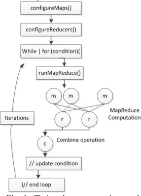
[image:3.612.357.496.256.450.2]There are many parallel algorithms with simple iterative structures. Most of them can be found in the domains such as data clustering, dimension reduction, link analysis, machine learning, and computer vision. These algorithms can be implemented with iterative MapReduce computation. Twister is a kind of iterative MapReduce model proposed by Indiana University. It is composed by several components, i.e. MapReduce main job, Map job, Reduce job, and combine job. Twister’s programming model can be described as in figure 1.
Fig. 1 Twister’s programming model
MapReduce jobs are controlled by the client node through a multi-step process. During configuration, the client assigns MapReduce methods to the job, prepares KeyValue pairs and prepares static data for MapReduce tasks through the partition file if required. Between iterations, the client receives results collected by the Combine method, and, when the job is done, exits gracefully. The message communicate between job is realized with message brokers, i.e. NaradaBrokering or ActiveMQ.
Reduce daemons operate on computation nodes. The number of reducers is prescribed in client configuration step. The reduce jobs depend on the computation results of Map jobs. The communication between daemons is through messages.
Combine job is to collect MapReduce results. It operates on client node. Twister uses scripts to operate on static input data and some output data on local disks in order to simulate some characteristics of distributed file systems. In these scripts, Twister parallel distributes static data to compute nodes and create partition file by invoking Java classes. For data which are output to the local disks, Twister uses scripts to gather data from all compute nodes on a single node specified by the user.
4 Parallel SVM based on Twister
4.1
Support Vector MachinesSVM first maps the input points into a high-dimensional feature space with a nonlinear mapping function and then carries through linear classification or regression in the high-dimensional feature space. The linear regression in high-dimension feature space corresponds to the nonlinear classification or regression in low-dimensional input space. The general SVM can be described as follows.
Let training samples be
, where , (classification)
or (regression), . Nonlinear
mapping function is .
Classification SVM can be implemented through solving the following equations.
min 𝑤,𝜉𝑖,𝑏�
1
2‖𝑤‖2+𝐶 � 𝜉𝑖 𝑖� 𝑠.𝑡.𝑦𝑖(Φ𝑇(𝑋
𝑖)𝑤+𝑏)≥1− 𝜉𝑖 ∀𝑖= 1,⋯,𝑛 (6) 𝜉𝑖≥0 ∀𝑖= 1,⋯,𝑛
By introducing Lagrangian multipliers, the optimization problem can be transformed into its dual problem.
min𝛼 � 𝛼𝑖𝛼𝑗𝑦𝑖𝑦𝑗𝑘(𝑥𝑖,𝑥𝑗) 𝑖,𝑗
− � 𝛼𝑖 𝑙
𝑖=1
𝑠.𝑡. 𝑦𝑇𝜶= 0 (7)
0≤ 𝛼𝑖<𝐶,𝑖= 1,⋯,𝑙
After obtaining optimum solution , the following decision function is used to determine which class the sample belongs to.
(8)
The classification precision of the SVM model can be calculated as
Accuracy =#correctly predicted data#total testing data × 100% It is very important to choose appropriate kernel function of SVM. The kernel function must satisfy the Mercer condition. At present, many kernel function model have been developed. Commonly used kernel functions include
(1) linear: 𝐾�x𝑖, x𝑗�= x𝑖𝑇x𝑗
(2) polynomial: 𝐾�x𝑖, x𝑗�=�𝛾x𝑖𝑇x𝑗+𝑟�𝑑,𝛾> 0 (3) radial basis function (RBF): 𝐾�x𝑖, x𝑗�=
exp (−𝛾�x𝑖−x𝑗�2),𝛾> 0
(4) sigmoid: 𝐾�x𝑖, x𝑗�= exp (−𝛾�x𝑖−x𝑗�2),𝛾> 0 Here, 𝛾,𝑟,𝑎𝑛𝑑𝑑 are kernel parameters.
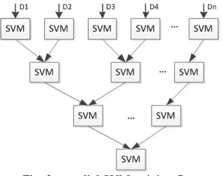
[image:4.612.358.516.440.565.2]The parallel SVM is based on the cascade SVM model. The SVM training is realized through partial SVMs. Each subSVM is used as filter. This makes it straightforward to drive partial solutions towards the global optimum, while alternative techniques may optimize criteria that are not directly relevant for finding the global solution. Through the parallel SVM model, large scale data optimization problems can be divided into independent, smaller optimizations. The support vectors of the former subSVM are used as the input of later subSVMs. The subSVM can be combined into one final SVM in hierarchical fashion. The parallel SVM training process can be described as in figure 2.
Fig. 2 parallel SVM training flow
vectors. In this paper, libSVM is adopted to train each subSVM.
4.2 Computation time analysis
The time cost of SVM can be divided into following sections. The computation time complexity of libSVM is 𝑂(𝑛2). The transformation time of data between Map and Reduce nodes is depend on the bandwidth of the connection network. The transfer time can be described as 𝑡𝑡𝑟𝑎𝑛𝑠. The combination time cost of two SVMs is 𝑂(𝑛). When training data set is divided into m ( m is the exponent value of 2) partitions, the computation cost is calculated as follows. The layers of cascade SVM is
𝑁= log2𝑚
Suppose that the ratio between the number of support vectors and that of whole training sample is 𝛼 (0 <𝛼< 1) and the ratio between support vectors and that of training sample except the first layer is 𝛽(1 <𝛽< 2), i.e. the number of the last layer in Fig. 2 is 𝑛𝑁=𝑛𝛼𝛽 and the number of training sample of the first layer is almost 𝑛1=𝑛/𝑚. The number of
training samples of the 𝑖 layer is 𝑛𝑖=𝑛𝛼𝛽 ∗ �𝛽 2�
𝑁−𝑖 . So the computation time can be calculated as follows.
𝑡=𝑂 ��𝑛 𝑚�
2
�+∑2 𝑂 ��𝑛𝛼𝛽 ∗ �𝛽2�𝑁−𝑖�2�
𝑖=𝑁 +
𝑂 �∑2 𝑛𝛼𝛽 ∗ �𝛽2�𝑁−𝑖∗2𝑁−𝑖
𝑖=𝑁−1 �+𝑡𝑡𝑟𝑎𝑛𝑠 (9) Overhead of data transfer mainly includes three parts. The first part is data transfer from Maptask nodes to Reducetask nodes. The transferred data are the support vectors obtained by Maptask nodes. The second part is data transfer from Reducetask nodes to server node. The transferred data is the support vectors also. The third part is the data transfer from server nodes to Maptask node. The transferred data is the training samples combined by two subSVM’s support vectors. The overhead of data transfer depend on the bandwidth of the MapReduce cluster.
From the architecture of parallel SVM, we can find that it is hierarchal structure. The low level SVM training has to be performed when all the upper level subSVM be trained. In the last level of the architecture, all the support vectors should be included in the training samples. The sample size must be bigger than the number of support vectors. When the ratio between support vector and training sample is bigger the speed up will be less. It is the shortcoming of the cascade SVM model.
5 Large scale classification based on
combination of parallel SVM and
interpolation MDS
The classification process based on combination of parallel SVM and interpolation MDS can be summarized as follows.
(1) Preprocess the collected sample data, i.e. normalization.
(2) Some samples are selected to be processed with MDS and the other samples are processed with interpolation MDS.
(3) The decreased samples are taken as the input of the SVM.
(4) Partition the samples into 𝑛 parts. Deploy the data to the computation nodes and create partition file. Samples are divided into two parts. One is to be used to train the SVM model. The other is used to test the trained model.
6 Examples
All examples are analyzed in India cluster node of
FutureGrid. Eucalyptus platform is adopted to configure the MapReduce computation environment. Twister0.9 software is deployed in each computation nodes. ActiveMQ is used as message broker. The configuration of each virtual machine is as follows. Each node is installed Ubuntu Linux OS. The processor is 3GHz Intel Xeon with 10GB RAM.6. 1 Adult data analysis 6.1.1 Data source
The source data are downloaded from NEC laboratory American Inc. website http://ml.nec-labs.com/download/data/milde/. In the adult database, 123 attributes are labeled 2 classes. Each attribute denoted by binary variable, i.e. 0 or 1. Labels are denoted by +1 or -1. It is a binary classification problem. The database includes two files. One is used for training and the other is used for testing. The training file includes 32562 samples. The testing file includes 16282 samples.
6.1.2 Dimension reduction
In this example, 4000 samples are selected to be mapped into low dimension space with MDS method. Firstly, calculate the distance matrix ∆. Euclidean distance is taken as the distance measure. The corresponding mapped vectors are calculated with MDS based on the distance matrix. The other samples are mapped into low dimension with interpolation MDS method. The number of nearest neighbor is set k = 10 . For comparison, the dimension number is set as 3, and 10 respectively.
6.1.3 Training process
comparison, the sample is partitioned into 1, 2, 4, 8 sub-samples respectively. The training and test result based on different partitions are listed in table 1, 2 and 3. Table 1 is based on the initial data without dimension reduction. Table 2 is based on the data whose features are reduced to 3 dimensions. Table 3 is based on the data whose features are reduced to 10 dimensions.
Table 1 analysis result of SVM with no dimension reduction
Number of nodes
Number of SVs
Training time(s)
Classification correct rate
1 11957 490.591 84.82
2 11933 281.152 84.98
4 11908 239.914 83.06
[image:6.612.72.276.184.409.2]8 11887 237.441 82.74
Table 1 analysis result of SVM with 3 dimensions Number
of nodes
Number of SVs
Training time(s)
Classification correct rate
1 5175 145.2 84.21
2 4956 80.871 84.27
4 4896 39.962 83.94
8 4826 31.696 83.79
Table 1 analysis result of SVM with 10 dimensions Number
of nodes
Number of SVs
Training time(s)
Classification correct rate
1 5137 227.88 82.76
2 6330 107.222 82.31
4 6122 97.51 81.66
8 5918 83.401 80.82
6.1.4 Results analysis
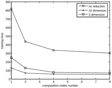
The analysis results are shown as in Fig.3 and Fig. 4. From Fig.3 we can find that the training time can be reduced greatly when the sample is partitioned 2 parts. But with the increase of partition number, the training time reduction will become slow. From Eq. (9), the computation cost mostly concentrate on the training calculation of each subSVM. The example was analyzed in HPC cluster. The data transfer time cost is minor. In this example, the ratio 𝛼 ≈0.35 and 𝛽 ≈1.2. The last layer will occupy the mainly part computation time and it will not decrease with the increase of partition number. With the decrease of 𝛼, the computation time can be reduced more. The training time can be decreased markedly when the feature vector is reduced with MDS method. Through the combination of parallel SVM and interpolation MDS, the training process time can be decreased markedly.
From figure 4 we can find the analysis correct rate will not decrease too much when it is analyzed with parallel SVM and MDS method.
[image:6.612.332.522.254.409.2]Fig. 3 Training time based on different partition nodes
Fig. 4 Correct rate based on different partition 6.2 Forest Covertype Classification 6.2.1 Data source
The source data are downloaded from
http://ftp.ics.uci.edu/pub/machine-learning-databases/covtype/. The data is used to classify forest cover type. The original data are collected by Remote Sensing and GIS Program, Department of Forest Sciences, College of Natural Resources, Colorado State University. Natural resource managers responsible for developing ecosystem management strategies require basic descriptive information including inventory data for forested lands to support their decision-making processes. The purpose is to predict the forest covertype according to cartographic variables’ values. The square of each observed section is 30 x 30 meter cell. There are 54 columns in each data item. They denote 12 variables, i.e. Elevation,Aspect,Slope,Horizontal_distance_to_hydr ology,Vertical_Distance_To_Hydrology,Horizontal_ Distance_To_Roadways,Hillshade_9am,Hillshade_N oon,Hillshade_3pm,Horizontal_Distance_To_Fire_P oints, Wilderness_Area, and Soil_Type, where Wilderness_Area is denoted by 4 binary columns and Soil_Type is denoted by 40 binary columns. They are labeled as 7 cover types, i.e. Spruce/Fir, Lodgepole Pine, Ponderosa Pine, Cottonwood/Willow, Aspen,
1 2 3 4 5 6 7 8
0 50 100 150 200 250 300 350 400 450 500
computation nodes number
tr
ai
ni
ng t
im
e
3 dimension 10 dimension no reduction
1 2 4 8
0 10 20 30 40 50 60 70 80 90 100
computation nodes number
c
o
rre
c
t ra
te
Douglas-fir, and Krummholz. There are 100000 samples in total. In this example, 40000 samples are taken as training samples and the left are taken as test samples.
6.2.2 Analysis preparation
In this example, 8 computation nodes are used. Training data are partitioned into n sections randomly. Each section has roughly equal number data. Each attribute is normalized according to the following equation.
Let attribute X denote attribute variable. The maximum value of X is 𝑥𝑚𝑎𝑥 and the minimum value is 𝑥𝑚𝑖𝑛. The range of normalized attribute is set [0, 1]. The normalized equation is
𝑥𝑛𝑜𝑟𝑚=𝑥𝑥 − 𝑥min 𝑚𝑎𝑥− 𝑥𝑚𝑖𝑛
6.2.3 dimension reduction
In this example, 4000 samples are selected to be pre-mapped into low dimension space. Firstly, calculate the distance matrix. Euclidean distance is adopted here. Then calculate the mapped vector according to the distance matrix with MDS method. The others are mapped into low dimension with interpolation MDS method. The number of nearest neighbor is set k = 10 . For comparison, the dimension number is set as 3 and 10 respectively.
6.2.4 Training process
The problem is taken as a multi-value classification problem. Multiclass classification is realized with pairwise method, i.e. k class SVM is realized through 𝑘(𝑘 −1)/2 binary SVMs. The “one against one” strategy, also known as “pairwise coupling”, “all pairs” or “round robin”, consists in constructing one SVM for each pair of classes. Thus, for a problem with k classes, k(k-1)/2 SVMs are trained to distinguish the samples of one class from the samples of another class. Usually, classification of an unknown pattern is done according to the maximum voting, where each SVM votes for one class.
In this example, C-SVC model is adopted. The parameter of the SVM model is set as follows. Constant C is set 1, radial basis function is taken as kernel function, and gamma is set as 0.01. Firstly, the example is analyzed with only 1 computation node, i.e. classical SVM method is used to train the SVM model. The trained model is used to predict the testing samples. The training time and classification correct rate are listed in Table 2. Secondly, the example is analyzed with the parallel SVM based on map/reduce. For comparison, the sample is partitioned into 2, 4, 8 sub-samples respectively. When the sample is partitioned into 2 sub-samples, 2 computing nodes are used. The training time and classification rate of each partition form based on
different feature dimensions are listed in table 4, 5 and 6.
Table 4 analysis result of SVM with no dimension reduction
nodes Number
Number of SVs
Training time(s)
Classification correct rate
1 15893 817.856 73.583
2 14904 435.674 72.26
4 14074 336.261 70.005
[image:7.612.334.533.110.342.2]8 13335 301.922 69.015
Table 5 analysis result of SVM with 10 dimensions nodes
Number
Number of SVs
Training time(s)
Classification correct rate
1 19072 126.354 71.755
2 18268 70.956 65.658
4 17553 57.628 64.338
8 16380 53.118 61.386
Table 6 analysis result of SVM with 3 dimensions nodes
Number
Number of SVs
Training time(s)
Classification correct rate
1 23646 247.805 72.813
2 23116 126.392 71.5866
4 22052 77.205 69.25
8 21204 69.472 68.866
6.2.5 Result analysis
This example is a multiclass classification problem. How to improve classification correct rate of multi-class is still a big problem. From Fig.5 we can find that the training time can be reduced greatly when the sample is partitioned 2 parts. But with the increase of partition number, the training time reduction will become slow. In this example, the ratio 𝛼 ≈0.4 and 𝛽 ≈1.2. It is similar to the analysis problem of example 1. But with the training time based on 10 dimensions is less than that based on 3 dimensions. It is perhaps that the training error can be met easily. The training time is less than that of no dimension reduction.
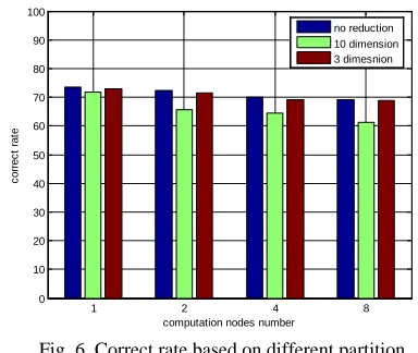
[image:7.612.333.523.547.697.2]From figure 6 we can find the analysis correct rate will not decrease too much when it is analyzed with parallel SVM and MDS method.
Fig. 5 training time based on different partition nodes
1 2 3 4 5 6 7 8
0 100 200 300 400 500 600 700 800 900
computation nodes number
tr
ai
ni
ng t
im
e
Fig. 6 Correct rate based on different partition
7 Conclusions
Data intensive data mining is still a big problems faced by computer scientist. SVM is taken as a most efficient classification and regression model. The computation cost of SVM is square proportion to the number of training data. Classical SVM model is difficult to analyze large scale practical problems. Parallel SVM can improve the computation speed greatly. In this paper, parallel SVM model based on iterative MapReduce is proposed. It is realized with Twister software. Feature extraction is an efficient means to decrease SVM training computation cost. Interpolation MDS is used to reduce the feature vector dimension. It is combined with parallel SVM. Through example analysis it shows that the combination of cascade parallel SVM based on Twister and interpolation MDS can reduce the computation time greatly. At the same time, the classification correct rate will not decrease. In total, the proposed classification method is efficient in data intensive problems.
Acknowledgements
This work is partially supported by Provincial Outstanding Research Award Fund for young scientist (No. BS2009DX016) and Provincial Fund for Nature project (No. ZR2009FM038).
References
[1] J R Swedlow, G Zanetti, C Best. Channeling the data deluge. Nature Methods, 2011, 8: 463-465.
[2] G C Fox, X H Qiu et al. Case Studies in Data Intensive Computing: Large Scale DNA Sequence Analysis. The Million Sequence Challenge and Biomedical Computing Technical Report, 2009
[3] X H Qiu, J Ekanayake, G C Fox et al. Computational Methods for Large Scale DNA Data Analysis. Microsoft eScience workshop, 2009
[4] J A Blake, C J Bult. Beyond the data deluge: Data integration and bio-ontologies. Journal of Biomedical Informatics, 2006, 39(3), 314-320.
[5] J Qiu. Scalable Programming and Algorithms for Data Intensive Life Science. Applications Data-Intensive Sciences Workshop, 2010
[6] R Guha, K Gilbert, G C Fox, et al. Advances in Cheminformatics Methodologies and Infrastructure to Support the Data Mining of Large, Heterogeneous Chemical Datasets. Current Computer-Aided Drug Design, 2010, 6: 50-67.
[7] C C Chang, B He, Z Zhang. Mining semantics for large scale integration on the web: evidences, insights, and challenges. SIGKDD Explorations, 2004: 6(2):67-76.
[8] G C Fox, S H Bae, et al. Parallel Data Mining from Multicore to Cloudy Grids. High Performance Computing and Grids workshop, 2008
[9] B J Zhang, Y Ruan et al. Applying Twister to Scientific Applications. Proceedings of CloudCom, 2010
[10] J Ekanayake, H Li, et al. Twister: A Runtime for iterative
MapReduce. The First International Workshop on
MapReduce and its Applications of ACM HPDC, 2010 [11] C. Cortes, V. Vapnik. Support Vector Networks. Machine
Learning,1995, 20: 273-297
[12] C C Chang, C J Lin. LIBSVM: a library for support vector machines. ACM Transactions on Intelligent Systems and Technology, 2011, 27(2): 1-27.
[13] B Boser, I Guyon, V Vapnik. A training algorithm for optimal margin classifiers. The 5th Annual Workshop on Computational Learning Theory, 1992.
[14] R E Fan, P H Chen, C J Lin. Working set selection using second order information for training SVM. Journal of Machine Learning Research, 2005, 6: 1889-1918.
[15] H P Graf, E Cosatto, et al. Parallel support vector machines: the Cascade SVM. Advances in Neural Information Processing Systems, MIT Press, 2005.
[16] K Woodsend, J Gondzio. Hybrid MPI/OpenMP parallel linear support vector machine training. Journal of Machine Learning Research, 2009, 10: 1937-1953
[17] J X Dong, A Krzyzak, C Y Suen. A fast Parallel Optimization for Training Support Vector Machine. Proceedings of 3rd International Conference on Machine Learning and Data Mining, 2003: 96—105.
[18] Jolliffe, I. T. Principal component analysis. New York : Springer, 2002.
[19] George K Matsopoulos. Self-Organizing Maps. INTECH, 2010.
[20] Borg Ingwer, Patrick J.F. Croenen. Modern
Multidimensional Scaling: Theory and Applications. New York : Springer, c2005. pp. 207–212
[21] Seung-Hee Bae, Judy Qiu, Geoffrey Fox. Adaptive Interpolation of Multidimensional Scaling International Conference on Computational Science ICCS Omaha Nebraska June 4-6 2012
1 2 4 8
0 10 20 30 40 50 60 70 80 90 100
computation nodes number
c
o
rre
c
t ra
te