Automatic, computer aided geometric design of free-knot, regression splines

City, University of London Institutional Repository

Citation

:

This is the unspecified version of the paper.

This version of the publication may differ from the final published

version.

Permanent repository link: http://openaccess.city.ac.uk/2368/

Link to published version

:

Copyright and reuse:

City Research Online aims to make research

outputs of City, University of London available to a wider audience.

Copyright and Moral Rights remain with the author(s) and/or copyright

holders. URLs from City Research Online may be freely distributed and

linked to.

City Research Online: http://openaccess.city.ac.uk/ [email protected]

Faculty of Actuarial

Science

and

Statistics

Automatic, Computer Aided

Geometric Design of

Free-Knot, Regression Splines

Vladimir K. Kaishev*, Dimitrina S.

Dimitrova, Steven Haberman and

Richard Verrall

Statistical Research Paper No. 24

August 2004

ISBN 1-901615-81-2

Cass Business School

106 Bunhill Row

London EC1Y 8TZ

Geometric Design of Free-Knot,

Regression Splines

by

Vladimir K. Kaishev

, Dimitrina S. Dimitrova, Steven Haberman

and Richard Verrall

Cass Business School, City University, London

Abstract

A new algorithm for Computer Aided Geometric Design of least squares (LS) splines with variable knots, named GeDS, is presented. It is based on interpreting functional spline regression as a parametric B-spline curve, and on using the shape preserving property of its control polygon. The GeDS algorithm includes two major stages. For the first stage, an automatic adaptive, knot location algorithm is developed. By adding knots, one at a time, it sequentially "breaks" a straight line segment into pieces in order to construct a linear LS B-spline fit, which captures the "shape" of the data. A stopping rule is applied which avoids both over and under fitting and selects the number of knots for the second stage of GeDS, in which smoother, higher order (quadratic, cubic, etc.) fits are generated. The knots appropriate for the second stage are determined, according to a new knot location method, called the averaging method. It approximately preserves the linear precision property of B-spline curves and allows the attachment of smooth higher order LS B-spline fits to a control polygon, so that the shape of the linear polygon of stage one is followed. The GeDS method pro-duces simultaneously linear, quadratic, cubic (and possibly higher order) spline fits with one and the same number of B-spline regression functions. The GeDS algorithm is very fast, since no deterministic or stochas-tic knot insertion/deletion and relocation search strategies are involved, neither in the first nor the second stage. Extensive numerical examples are provided, illustrating the performance of GeDS and the quality of the resulting LS spline fits. The GeDS procedure is compared with other existing variable knot spline methods and smoothing techniques, such as SARS, HAS, MDL, AGS methods and is shown to produce models with fewer parameters but with similar goodness of fit characteristics, and visual quality.

Keywords: spline regression, B-splines, Greville abscissas, CAGD, free-knot splines, control polygon

1. Introduction.

Consider a response variable y and an independent variable x, taking values within a certain interval @a,bD and assume there is a functional relationship between x and y of the form

(1)

y= fHxL+ e,

where fHÿL is an unknown function and e is a random error variable with zero mean. A problem which arises in a number of statistical applications is to estimate fHÿL, based on a sample of observations 8yi, xi<i=1

N _.

Different nonparametric smoothing methods for the solution of this problem have been proposed and the related literature is extensive. We will mention here some well known, spatially adaptive smoothing techniques such as: the wavelet shrinkage methods of Donoho and Johnstone (1994, 1995), the variable bandwidth kernel method of Fan and Gijbels (1995), hybrid adaptive splines (HAS) of Luo and Wahba (1997). Another popu-lar approach to smoothing is to use penalized splines, considered by Eubank (1988), Wahba (1990), Marx and Eilers (1996), Rupert and Carroll (2000), Rupert (2002). A third class of methods uses adaptive knot selection procedures, such as stepwise knot inclusion/deletion strategies, to develop variable knot spline regression models. Among the latter are the early work of Smith (1982), the TURBO spline modelling technique of Friedman and Silverman (1989), the MARS method proposed by Friedman (1991), the POLYMARS of Stone et al. (1997), and more recently the minimum description length (MDL) regression splines of Lee (2000) and the spatially adaptive regression splines (SARS) of Zhou and Shen (2001). A different knot removal algorithm for constructing splines with "almost free" knots, chosen from a subset of the data points, was proposed by Lytch and Mørken(1993). Constructing multivariate spline regression and knot loca-tion was considered also by Kaishev (1984). A fourth group of works applies reversible jump Markov chain Monte Carlo (RJMCMC) based methods, to develop Bayesian adaptive splines, such as those of Smith and Kohn (1996), Denison at al. (1998) and Biller (2000), in the context of generalized linear models. These procedures simulate tens of thousands of spline models which are then averaged pointwise to produce a resulting estimate of f, but they are associated with a high computational cost and the inconvenience of having the resulting model in a non-explicit form. A stochastic optimi-zation algorithm for "almost free"-knot splines, called adaptive genetic splines (AGS) was recently proposed by Pittman (2002) but the related computational cost is also a concern, as noted by the author.

De Boor, 2001) and by Jupp (1978). As is well known, the non-linear optimization problem of finding the best least squares free-knot spline approximation may not have a unique solution, and as noted by Jupp (1978), may have potentially a high number of local extrema. The routine of De Boor and Rice (1968), called NEWNOT leads to a possibly locally optimal knot placement, given the number of knots is known. The LS approximation with as few knots as possible has been considered by Hu (1993) and by Schwetlick and Schütze (1995), who combine non-linear optimization with a knot removal and relocation strategy. Reported numerical examples and computer times refer to models with only a small number of knots. However, the computational cost of run-ning such routines may be prohibitive if splines with many more knots are required to fit very unsmooth functions, based on large data sets, such as the HeaviSine, Doppler, Bumps and Blocks examples. The latter were first introduced by Donoho and Johnstone (1994) and are considered here as test examples 4-7 in Section 6. A recent account of free-knot least squares splines and knot selection strategies is provided by Cox et al. (2002).

In conclusion, we note that most of the quoted spline fitting methods of the third and fourth group perform knot placement search, within suitable subsets of candidate knot locations, e.g. the data points 8xi<iN=1, and hence are not entirely free-knot splines. They

apply either deterministic or stochastic adaptive knot insertion/deletion and relocation strategies, which may suffer from the knot confounding problem, as noted by Zhou and Shen (2001). Moreover, they may become computationally prohibitive for highly unsmooth functions and large data sets (see e.g. Lee 2000). Another drawback of the above mentioned algorithms is that most of them involve parameters whose values need to be subjectively preassigned by the user. For example, in some cases a guess for an initial set of knots is needed or the user is required to set lower and upper bounds for the number of knots to be included in the final fit. However, such choices may significantly affect the performance of the corresponding algorithms and the quality of the resulting fits. A further problem is that some of the methods impose limitations on the data set, e.g., need rescaling so that xiœ@0, 1D, i=1, ..., N. The wavelet shrinkage method of

Donoho and Johnstone (1994) requires equally spaced 8xi<iN=1 with N =2i, i=1, 2, ....

All of the above mentioned procedures do not allow real time, visual control of the entire fitting process, which is a desirable feature in many of the practical applications. As will be seen, the method developed here overcomes the problems that have been identified.

curves through scattered points on the plane, in Computer Aided Geometric Design (CAGD) applications. As a consequence, our algorithm is very fast, since there is no computationally expensive stochastic or deterministic knot relocation search involved. In order to distinguish the splines produced by this new method from MARS, TURBO splines, POLYMARS, HAS, SARS, AGS, NEWNOT etc, we call our procedure, the method of geometrically designed (GeD) splines, or GeDS in abbreviated form.

We will show that the proposed method of constructing GeD splines may be equally successfully applied to recover both smooth or wiggly functions with highly non-homoge-neous smoothness properties over thex range. By recovering f, we mean reproducing it, not only sufficiently accurately (with respect to the related mean squared error), but also with the corresponding estimated curve having desirable visual characteristics. As will be illustrated, our method produces good estimates with an appropriate degree of smooth-ness, avoiding overfitting or underfitting, for widely varying signal-to-noise ratios. The method is also automatic, since in most of the applications the user needs to input only the data set 8yi, xi<iN=1 and run the corresponding code. It is simple, i.e., easy to

imple-ment and follow by users with different backgrounds, allowing them to have visual control and understanding of the fitting process and the corresponding output. Finally, we note, that the GeDS method gives rise to a very fast computational algorithm, taking just seconds on a standard PC to recover f , even if it is highly unsmooth and the result-ing spline fit involves many knots. We do not aim at necessarily findresult-ing spline fits with as few knots as possible, and with optimal knot placement. However, in most of the examples presented in Section 6, the resulting GeD splines have very few knots, produc-ing very low mean squared error (MSE), within the noise level. In the case of the well known Titanium Heat data example, first given in De Boor and Rice (1968) (see our Example 8, Section 6), the MSE of the GeD quadratic spline fit is lower than that for the optimal cubic fit, found by Jupp (1978), both fits having five internal knots.

2. The B-spline regression as a parametric curve

As mentioned earlier, we base our approach to constructing GeD splines on the idea that fitting a variable knot, least squares spline regression to a noisy set of data 8yi, xi<iN=1

may be viewed as a process of computer aided geometric design of the shape of a two dimensional parametric curve, guided by the data points whose "true" location on the plane is perturbed by the noise component e. To elaborate further on this idea, recall that a two dimensional parametric curve QHtL in CAGD is given coordinate-wise as

QHtL=9xHtL yHtL=,

where t is a parameter , tœ @a,bD.

Let us note, that the functional dependence underlying (1) is in fact a functional curve of the form y= fHxL that can be viewed as a special case of a parametric curve for which

xHtL=t, i.e.,

QHtL=9xHtL yHtL==9

t fHtL=.

In this paper we assume that f is a spline function of degree n-1(order n), defined on @a,bD, which can be represented as an appropriate linear combination of B-splines of order n. The latter are piecewise polynomial functions of degree n-1, defined on the set of knots Dk,n=8ti<i=1

2n+g1+...+gk

, with

(2)

t1§t2§...§tn-1§tn<tn+1= ...=tn+g1 <tn+g1+1= ...=tn+g1+g2 <

...<tn+g1+...+gk-1+1= ...=tn+g1+...+gk <tn+g1+...+gk+1§...§t2 n+g1+...+gk,

where tn=a, tn+g1+...+gk+1=b, and 1§gi§n-1, i=1, ...,k are called the

multiplici-ties of the knots. B-splines coincide with a polynomial of degree n-1 at each of the intervals between adjacent, distinct knots and these pieces are smoothly joined at the latter knots, up to their Hn-1-giL-th derivative. In this paper we will use splines with

simple knots (of multiplicity one, i.e., gi=1, i=1, ..., k) except for the n left and right

most knots which will be assumed coalescent. In this case (2) simplifies to

(3)

Dk,n=8t1=t2= ...=tn<tn+1<...<tn+k<tn+k+1= ...=t2 n+k<.

Denote by SDk,n the linear space of all n-th order spline functions defined on Dk,n. In

order to express a spline f œSDk,n, one can introduce p= n+g1+...+gk B-splines

Ni,nHtL, i=1, ..., p, of order n on Dk,n, defined through the Mansfield-De Boor-Cox

recurrence relation

(4)

Ni,0HtL=9

1 0

if

(5)

Ni,nHtL=ÅÅÅÅÅÅÅÅÅÅÅÅÅÅÅÅÅÅ_ti+nt-_-1ti_-ti Ni,n-1HtL+ ÅÅÅÅÅÅÅÅÅÅÅÅÅÅÅÅÅÅ_tit₊i_n+_-n-_ti+t₁ Ni+1,n-1HtL.

Using B-splines defined on Dk,n, one can approximate fHxL with a spline function

(6)

fDk,nHxL=q'NnHxL=⁄i=1

p _q

iNi,nHxL,

where q=Hq1, ... qpL' is a vector of unknown parameters, to be estimated and

NnHxL=HN1,nHxL, ..., Np,nHxLL'.

If n, k and Dk,n are known, one can estimate q based on 8yi, xi<iN=1 using the least squares

method as

q` =_HF'FL-1F'Y,

where F =HNnHx1L, ..., NnHxNLL', Y =Hy1, ..., yNL', and F ' F is non-singular, i.e., the

Schoenberg-Whitney condition holds. The latter condition states that F ' F is non-singu-lar iff each interval @ti,ti+nD contains at least one observation xi, i.e., there exist indexes

1§l1<l2< ...<lp§N, such that ti<xli<ti+n, i=1, ..., p. Thus, the LS regression

spline fit for a fixed Dk,n is

f`_Dk,nHxL=‚

i=1 p

q`iNi,nHxL.

However, the degree n-1, the number of knots k and their position in Dk,n are in

gen-eral also unknown parameters which need to be determined. As mentioned earlier, such splines are called splines with free or variable knots, for which one of the most impor-tant problems is to define the number and location of the knots. In Section 3, we will present an algorithm for the solution of this problem, approaching the regression spline (6) as a parametric curve. Thus, if we view the functional B-spline curve (6) as paramet-ric, we can write

(7) QHtL=9xHtL

yHtL==9 t fDk,nHtL=

=9 t

⁄i=1

p _q

iNi,nHtL

=.

To develop the GeD spline methodology we will need some of the properties of the B-splines, which have made them the preferred set of basis functions in CAGD, approxi-mation theory and statistics. The first such property of crucial importance for CAGD applications is the partition of unity property.

Property 1 (partition of unity). The sum of all B-splines evaluated at t is equal to one,

i.e.,

⁄i=j-n+1 j

Ni,nHtL=1, for any tœ@tj,tj+1L, j=n, ... , n+k.

Proof. See, for example De Boor 2001, p. 96. Ñ

Property 2 (linear precision). The following identity holds

(8)

t=⁄_ip=1x*i Ni,nHtL ,

where,

(9)

x_i*_=Ht

i+1+...+ti+n-1L ê Hn-1L, i=1, ..., p.

Proof. The result follows from Marsden's identity (see e.g. Cohen et al. 2001, Theorems

7.19, 7.14). Ñ

The values xi* given by (9) are known as the Greville abscissas. In view of the linear

precision property (8) we can rewrite (7) as

(10) QHtL=9xHtL

yHtL==9 t fDk,nHtL=

=9⁄i=1

p _x

i*Ni,nHtL

⁄i=1

p _q

iNi,nHtL

=.

Note that (10) is a subset of the general class of parametric B-spline curves

(11) QHtL=⁄_ip₌₁ ciNi,nHtL=9

⁄i=1

p _x

iNi,nHtL

⁄i=1

p _q

iNi,nHtL

=,

where ci=Hxi,qiL, i=1, ..., p, denote the vertexes of the control polygon C, of QHtL,

called also the control points of QHtL. Note that, due to the partition of unity property of B-splines, any point from a B-spline curve QHtL in (11) is expressed as a convex, barycen-tric combination of its control points. This leads us to Property 3.

Property 3 (affine invariance). The parametric B-spline curve QHtL is affinely invariant.

Proof. The proof follows by the definition of affine invariance (see e.g. Farin 2002). Ñ

We note that QHtL are also invariant under an affine reparametrization, a property which, as a consequence, holds for GeDS.

Since the set of curves, defined by (10), is a subset of the parametric B-spline curves in (11), each one of them has a control polygon with vertexes Hx_i*,qiL, i.e.,

(12) QHtL=⁄_ip₌₁ ciNi,nHtL=9

⁄i=1

p _x

i*Ni,nHtL

⁄i=1

p _q

iNi,nHtL

=.

A functional B-spline curve QHtL of order n=3 and its control polygon C are illustrated in Fig. 1. Let us note that the control polygonplays an important role in CAGD since it mimics the shape of its related curve. This is stated by the following property.

Property 4 (shape preserving). The B-spline curve QHtL has the same shape as its

control polygon, i.e, it crosses any straight line no more often than does C.

Proof. The result follows by applying the well known Schoenberg's variation

not bigger than the number of sign changes in the sequence of its B-spline coefficients

qi, i=1, ..., p (see e.g., De Boor 2001, p. 141). Ñ

In particular, in the linear case Hn=2L, QHtL coincides with its control polygon and hence the shape preserving property holds exactly. In the quadratic case Hn=3L the curve QHtL, evaluated at the knots t3,t4, ..., tk+4, interpolates C and is tangential to each

of its segments, ci,ci+1, dividing it in a proportion Hti+2-ti+1L:Hti+3-ti+2L,

i=2, ...,k+2. This is illustrated by Fig. 1, in the case of k =5, where Dj=tj+1-tj,

j=3, ...k+3. In the cubic case Hn=4L, the spline curve, evaluated at a knot, i.e., QHti+3L is somewhere within the triangle of points ci, ci+1 ci+2, i=1, 2, ..., p. Hence, the

higher the degree, the stronger the curve deviates from its control polygon C, but it still remains within the convex hull of C, due to the following property.

Property 5 (convex hull). The B-spline curve QHtL lies within the convex hull of its

control polygon, and more precisely, each of its polynomial segments lies within the convex hull of the n control points, defining it.

Proof. The proof follows from the fact that every point of the curve QHtL of order n is a

barycentric combination of n control points, i.e., QHtL=⁄i=j n+j-1

ciNi,nHtL,

tœ@tn+j-1,tn+jD, j=1, ...,k+1. Ñ

The shape preserving and convex hull properties, illustrated in Fig. 1 are an important motivation for developing the GeDS algorithm. The shaded areas in Fig. 1 are examples of convex hulls in the case of a quadratic B-spline curve.

x1*

t1=t2=t3

a

x₂* _x

3

* _x

4

* _x

5

* _x

6

* _x

7

* t4 t5 t6 t7 t8 x8*

t9=t10=t11

b

q1=q8

q2

q3=q4

q5

q6

q7

D6 D7 D8

c1

c2

c3 c4

c5

c6

c7

c8

D6:

D7

D₇

:_D

8

Fig. 1. A quadratic, functional B-spline curve and its control polygon.

the same time being tangential to each of the segments of its control polygon. This makes quadratic splines especially suitable for implementing the GeDS algorithm.

Thus, due to the shape preserving and convex hull properties, the control polygon can be manipulated in order to design the shape of a functional or parametric B-spline curve. We use this approach in solving the problem of recovering the unknown function f

from a set of observations 8yi,xi<iN=1 and construct an appropriate control polygon C

which captures the shape of the data. Then, having C and the relation between ci and ti,

given by (9), we define the number and position of the knots of a smooth B-spline curve, which best approximates the data in the LS sense. The procedure of finding the most appropriate control polygon C is the first major stage of our algorithm, explained in details in Section 5. The problem of defining the number and position of the knots of a functional B-spline curve, given its control polygon, comprises the second major stage of the algorithm.

Let us note that, for the functional curves (12), given the knots Dk,n and the degree

n-1, it is always possible to use (9) and find values of the Greville abscissae x_i*. Then, the free parameters to be estimated, based on the data are the y-coordinates of the con-trol points. The latter, called De Boor ordinates, coincide with our unknown spline regression coefficients q, as seen from (12). Hence, given n and Dk,n, finding LS

esti-mates of the regression coefficients q, based on 8yi, xi<iN=1, is equivalent to estimating the

location of the y-coordinates of the vertexes of the control polygon in (12). This is an important point, which, along with the other recollected properties of B-spline paramet-ric curves, has allowed us to develop our CAGD approach to constructing free-knot least squares regression splines.

To implement the proposed approach, given a control polygon C and a fixed n, we need to be able to find Dk,n of the functional B-spline curve, attached to it. Hence, given the

control points ci, if their x-coordinates xi could be obtained as the Greville abscissa

values from an appropriate set of knots Dk,n, one could attach a functional B-spline

curve fDk,n, on to the polygon C, since the linear precision property (8) will be fulfilled.

Let us note that conditions (9) are imposed, since we are interested in modeling func-tional curves in a parametric form. However, for parametric curves, (9) is not required. So, one can arbitrarily choose the set of knots and attach more then one parametric B-spline curve on to a given control polygon.

Unfortunately, it is not always possible to find the knots Dk,n, given the x-coordinates,

xi, of the control points, so that (9) is satisfied. It can be seen that expressions (9) form

an over-determined system of equations, with constraints on the knots, given by the definition of Dk,n. Since x1=a and xp=b, the system (9) contains k+n-2 equations

and k ordered, unknown knots. In the next section we propose a method, which over-comes this difficulty and expresses the set of internal knots, through xi, i=1, ..., p, so

3. Positioning of the knots

In this section, we present a method, called averaging knot location method. It allows to avoid the problem of solving system (9) with respect to ti+n, i=1, ..., k and at the same

time provides a set of knots Dk,n, such that the B-spline curve fDk,n approximately obeys

the linear precision property (8). This implies that, for given xi of C, the averaging knot

location method produces Dk,n, such that the Greville abscissas xi*, obtained from Dk,n,

are very close to xi of C.

1) The averaging knot location method

Choose the internal knots in Dk,n as the averages of the x-coordinates of the vertexes of

the control polygon C, i.e.,

(13)

ti+n=Hxi+1+...+ xi+n-1L ê Hn-1L, i=1, ... ,k.

The following proposition establishes an important property of rule (13), which will be used throughout the sequel.

Proposition 1. The averaging knot location method (13) is affinely invariant.

Proof. Note that, according to (13), an internal knot ti+n is a convex, barycentric

combina-tion of xi+1, ... , xi+n-1. Hence, the assertion of the proposition follows, since affine

transformations leave barycentric combinations invariant. Ñ

Now, we investigate the extent to which the averaging knot location method preserves the linear precision property (8).

Proposition 2. The deviation dHtL:= » ⁄_ip₌₁x_i*Ni,nHtL-⁄i=1

p _x

iNi,nHtL » of the spline

function ⁄_ip₌₁xiNi,nHtL, with knots given by (13), from the straight line tª⁄i=1

p _x

i

*_N

i,nHtL,

tœ @a,bDis bounded by

(14)

d_HtL§maxjœ82,...,p-1< »x*j- xj».

Proof. Note that

dHtL= » ⁄_ip₌₁Hx_i*- xiLNi,nHtL » §⁄i=1 p _{» Hx}

i

*_{- x}

iLNi,nHtL »

§maxjœ82,...,p-1<»x*j- xj» ⁄i=1 p

Ni,nHtL§maxjœ82,...,p-1< »x*j- xj»

where we have applied the partition of unity property of Ni,nHtL, i=1, ..., p. Ñ

In order to assess the accuracy of the bound (14) and illustrate the extent to which the averaging knot location method preserves the linear precision property of B-spline curves, we have randomly generated abscissa values xj for three fixed numbers of

thousand graphs of ⁄_ip₌₁xiNi,nHtL, tœ @0, 1D with knots defined by (13), have been

plotted in Fig. 2 (a), (b) and (c).

0.2 0.4 0.6 0.8 1

HaL k=3

0.2 0.4 0.6 0.8 1

0.2 0.4 0.6 0.8 1

HbL k=8

0.2 0.4 0.6 0.8 1

0.2 0.4 0.6 0.8 1

HcL k=20

0.2 0.4 0.6 0.8 1

Fig. 2. Graphs of 1000 simulations of ⁄_ip₌₁xiNi,nHtL, with Dk,3 according to (13)

and estimates of d`<sub>0.95</sub>max and b`_0.95max for (a) p=6 Hk =3L, d`<sub>0.95</sub>max=0.16, b`_0.95max =0.31; (b) p=11 Hk=8L, d`<sub>0.95</sub>max=0.09, b`_0.95max =0.17; (c) p=23 Hk =20L, d`_0.95max=0.05,

b`_0.95max =0.09.

In Fig. 2, two corridors are also shown. The first, defined by the dashed lines, is based on the 95 sample percentile of the maxt dHtL, denoted by d

`

0.95 max

. The second corridor (the solid lines) is based on the bound (14), denoted by b`_0.95max. As can be seen from Fig.2, the maximum deviation of ⁄_ip₌₁xiNi,nHtL from the straight line t is reasonable, and decreases

as the number of knots increases. Thus, the higher the number of knots, the better rule (13) allows for the linear precision property of a B-spline curve to be preserved. Similar conclusions are found to hold for the cubic case (n=4), applying both d`<sub>0.95</sub>max and b`_0.95max. We have explored also other possible methods for defining the knots through the coordi-nates of the control points ci, i=1, ..., p. In order to formulate these methods, we have

applied ideas which are similar to those used in CAGD to define rules for choosing parameter values, that correspond to some points on the plane, to be interpolated by a parametric B-spline curve. In this case, several alternative methods, such as the uniform, the chord length, and the centripetal methods have been proposed in the CAGD litera-ture (see Farin 2001). According to these methods, the parameter values are chosen to be proportional to the distances between the data points which are interpolated. However, our purpose here is different, in that we seek to express the knots of a functional B-spline curve which approximates a set of data through the control points. So, we define the following alternatives to the latter methods.

2) The uniform method

(15)

ti+n=a+i ÅÅÅÅÅÅÅÅÅÅ_kb₊₁-a, i=1, ..., k 3) The "Chord Length" method

(16)

ti+n=a+Hb-aL HÅÅÅÅÅÅÅÅÅÅÅÅÅÅÅÅÅÅÅÅÅÅÅÅÅÅÅÅÅÅÅÅLi+1+...+_n-1Li+n-1L êL, i=1, ..., k,

where L=⁄p_j=2∞cj-cj-1¥=‚ j=2

p "#################################################

and Ll=⁄lj=2∞cj-cj-1¥, l=2, ..., p-1. 4) The "Centripetal" method

(17)

ti+n=a+Hb-aL HÅÅÅÅÅÅÅÅÅÅÅÅÅÅÅÅÅÅÅÅÅÅÅÅÅÅÅÅÅÅÅÅLi+1+...+_n-1Li+n-1L êL, i=1, ...,k,

where L=⁄p_j=2H∞cj-cj-1¥L0.5 and Ll=⁄lj=2H∞cj-cj-1¥L0.5, l=2, ..., p-1.

We have investigated these three rules, as alternatives to the averaging knot location method. Their ability to preserve the linear precision property (8) is illustrated in Fig 3. A comparison of Fig. 3 with Fig. 2 (c), shows that these methods are considerably worse than the averaging knot location method. Note, that rules 2) and 3) are not affine invari-ant and use both the x and y coordinates of ci, in contrast to the averaging knot location

method, which is affine invariant and uses only the x-coordinates xi, i=1, ..., p of the

vertexes of C.

0.2 0.4 0.6 0.8 1

HaL k=20

0.2 0.4 0.6 0.8 1

0.2 0.4 0.6 0.8 1

HbL k=20

0.2 0.4 0.6 0.8 1

0.2 0.4 0.6 0.8 1

HcL k=20

0.2 0.4 0.6 0.8 1

Fig. 3. Graphs of 1000 simulations of ⁄_ip₌₁xiNi,nHtL for p=23 Hk=20L with Dk,3

defined according to: (a) the uniform method (15), d`<sub>0.95</sub>max =0.28, b`_0.95max =0.29; (b) the chord length method (16), d`<sub>0.95</sub>max=0.31, b`_0.95max =0.32; (c) the centripetal method (17), d`<sub>0.95</sub>max=0.27, b`_0.95max =0.28.

4. The GeDS algorithm

We transfer these CAGD ideas to the context of non-parametric regression smoothing, in order to develop our new method for the construction of "geometrically designed", free knot, least squares B-spline regression curves, i.e., GeDS. The method includes two major stages, A and B. In stage A, a LS linear spline fit is constructed, in order to obtain the "geometric form" of the data. For this purpose, a new, spatially adaptive procedure for automatic knot insertion, equipped with an appropriate stopping rule, is introduced. The LS linear fit is then used in stage B as a guideline for designing the shape of a smoother, quadratic, cubic (or higher order) LS spline model. We note that the knots are determined as the averages of the knots of the linear spline fit, applying (13). This distin-guishes our GeDS algorithm from other existing spline methods and makes it very fast, since no time consuming, knot insertion-deletion schemes, or other simulation and search algorithms are involved. As will be seen from the examples, stages A and B are sufficient to obtain an accurate fit to the data.

In what follows, we give further details of the two stages of the proposed procedure for constructing GeDS.

Stage A. Construction of a free knot, LS linear B-spline fit by an automatic knot

insertion algorithm.

In this first stage, an automatic knot insertion algorithm is applied to construct a free-knot, least squares, linear (order n=2) B-spline curve (polygon), which reproduces the "shape" of the data set 8yi,xi<iN=1. The algorithm may be given the following geometric

interpretation. It starts from an LS fit, in the form of a straight line segment. The latter is then sequentially "broken" into a piecewise linear LS fit, by adding knots, one at a time, at some points, where the fit deviates most from the "shape" of the data, according to a measure based on appropriately defined clusters of residuals. A stopping rule is intro-duced, which allows us to determine the appropriate number and location of the knots of the linear spline fit and thus, avoid over- or under-fitting. Note that the LS linear B-spline fit f`_Dk,2HxL, produced in this way, coincides with its control polygon, hence its knots Dk,2 coincide with the abscissas of its control points, i.e., ti+1= xi, i=1, ..., p,

p=k+2. So, as it will be illustrated in the next section, the linear GeD spline fit

f`_Dk,2HxL is a sufficiently accurate reconstruction of the unknown function, given that no further smoothness is required. If a smoother fit is required, a higher order GeD spline is constructed in stage B of the GeDS procedure. A formal description of the algorithm for stage A is given in Section 5.

Stage B. Designing the shape of a higher order (quadratic, cubic etc.) LS spline curve,

via the LS B-spline polygon of stage A.

For n=3, 4, ... we apply the averaging knot location method (13), and choose the k

internal knots ti+n, i=1, ...,k in Dk,n, as the averages of abscissa values xi+1,

Based on Dk,n we then construct a higher order (quadratic, cubic etc.) LS B-spline

regres-sion curve, f`<sub>Dk,n</sub>HxL, fitting the data. The latter fit has a control polygon with vertexes, whose y-coordinates are the LS regression estimates q`i, i=1, ..., p and whose x

-coordi-nates are the Greville abscissas x_i*, obtained from the knots Dk,n, applying (9). We note

that the p vertexes of the two polygons, the control polygon of the LS higher order B-spline fit f`<sub>Dk,n</sub>HxL, and the LS linear B-spline fit, f`_Dk,2HxL, will be correspondingly close to each other. Their x-coordinates xi and xi* are close, due to the linear precision

property of the averaging knot location method (see Fig 2). Their y-coordinates, f`_Dk,2HxiL

and q`i, are close, since f

`

Dk,2HxiL and f

`

Dk,nHxi

*_{L are close as LS fits to 8y}

i, xi<iN=1, evaluated

at the close x locations xi and xi*, and f

`

Dk,nHxi

*_{Lº q}`

i. For a proof of the fact that

f`<sub>Dk,n</sub>Hx<sub>i</sub>*Lº q`i see e.g., Cohen et al. (2001), p. 281.

In this way, we assure that the control polygon of f`<sub>Dk,n</sub>HxL is close to the LS B-spline polygon f`_Dk,2HxL. But, due to its shape preserving property (see Section 2), the fit f`_Dk,nHxL

will have the same shape as its control polygon, hence will be close to the shape of the LS B-spline polygon f`_Dk,2HxL, which follows the shape of the data. But since, applying the averaging knot location method (13), more knots are inserted at locations where

f`_Dk,2HxL is more wiggly and less knots at its smoother segments, we guarantee that more knots are placed where the data exhibits more variation. In this way we assure that

f`_Dk,nHxL has appropriately located set of knots and adequately approximates the data. This is the basic CAGD idea underlying stage B of the proposed GeDS method. It allows us to avoid complex and time consuming knot optimization procedures. As will be illustrated by the examples in Section 6, the resulting fits have good visual quality and appropriate goodness of fit measure.

Remark: Stages A and B are sufficient to produce a very good quality spline fit with a

reasonably small number of knots as seen from the examples, given in Section 6. How-ever, since GeDS does not produce optimally placed knots, in some applications, a Fibonacci optimization search applied sequentially to each knot, produced after Stage B, may give some improvement of the MSE (see Example 8, Section 6).

5. An automatic, knot insertion algorithm for free-knot, LS linear

B-spline regression

In view of the importance of stage A of GeDS, this section contains a detailed descrip-tion.

Step 1. Set n=2 and k=0, i.e, the starting set of knots is D0,2 =8ti<i4=1 with

t1= t2=a<b=t3= t4 and find the LS B-spline fit, in the form of the straight line

f`<sub>D0,2</sub>HxL= q`1N1,2HxL+q

`

Find the residuals riªrHxiL= yi- f

`

D0,2HxiL, i=1, ..., Nand calculate the residual sum of

squares RSSHkL=⁄_iN₌₁r2_i and the mean squared error MSEHkL=RSSHkL êN of the fit with k internal knots. Since the i-th residual rHxiL, is a function of xi, i=1, 2, ..., N we

will refer to xi as the x-value of the i-th residual.

Step 2. Group the consecutive residuals ri, i=1, ..., N into clusters by their sign, i.e.,

find a number l, 1§ l§ Nand a set of integer values dj>0, j=1, ..., l such that

signHr1L= ...=signHrd1L∫signHrd1+1L=signHrd1+2L= ...=signHrd1+d2L∫

...∫signHrd1+d2+...+dl-1+1L=signHrd1+d2+...+dl-1+2L= ...=signHrd1+d2+...+dlL,

and ⁄l_j=1dj=N. Note that the clusters are formed and numbered consecutively,

follow-ing the order of the residuals, i.e., the order of their x-values x1<x2<...<xN.

Step 3. For each of the l clusters of residuals of identical signs, calculate the

"within-clus-ter" mean residual value

mj=

i

k jjjjj j‚

i=1

dj

rdHjL+i

y

{ zzzzz

z ìdj, j=1, ... ,l,

where dHjL=d1+d2+...+dj-1 and the "within-cluster" range xj, defined as the

differ-ence between the right-most and the left-most x-value of the residuals, belonging to the

j-th cluster, i.e., xj=xdHj+1L-xdHjL+1, j=1, ...,l. Throughout the sequel, we will need

the more general notation for dHjL=⁄_i<jdi to denote partial sums of non-ordered values

di, for which i< j and we will call the interval between the right-most and the left-most

x-value of the residuals, belonging to the j-th cluster, i.e., @xdHjL+1,xdHj+1LD, the

"within-cluster" interval.

Step 4. Find

(18)

mmax = max

1§j§lHmjL

(19)

xmax= max

1§j§l HxjL

and calculate, correspondingly, the normalized "within-cluster" mean and range values

m£_j=mjêmmax and x£j= xjêxmax, so that0<m£j§ 1, 0< x£j§ 1. Note that the equalities

(18) and (19) will not necessarily be fulfilled for one and the same cluster index j, i.e., the two maximums mmax and xmax may in general be attained for 2 different clusters

with indexes jm∫ jx.

Step 5. Calculate the cluster weights

(20)

wj= bm£j+H1- bLx£j, j=1, ... ,l,

where, b is a real valued parameter, 0§ b §1. The value wj can serve as a measure,

Obviously, the weight wj itself is a weighted sum of the normalized "within-cluster"

mean and "within-cluster" range values and the weight b is one of the parameters, whose value will need to be chosen by the user at the start of Stage A.

Step 6. Order the clusters in descending order of their weights wj, j=1, ... ,l, i.e.,

create a list of corresponding cluster indexes 8j1, j2, ... , jl< such that

wj1¥wj2 ¥...¥wjl. In the case where some clusters have coincident weights, they are

ordered in descending order of their "within-cluster" means. If the latter coincide, the order between the clusters is set, according to the descending values of the "within-clus-ter" ranges. In the case of coincident "within-clus"within-clus-ter" ranges, the clusters are ordered with respect to the number of residuals (of identical sign) in each cluster. Finally, if all of the listed characteristics of some of the clusters are identical, they are ordered in decreasing order with respect to the x-value of the right most residual in the cluster. These proposed ways of ordering the clusters are reasonable and meaningful, since they all characterize, in one way or another, how much the current least squares linear spline fit f`<sub>Dk,2</sub>HxL deviates from each of the clusters. Thus, to improve f`_Dk,2HxL, we insert a new knot, at an appropriate location, in the "within-cluster" interval of x-values, correspond-ing to the j1-th cluster. Since, in general, even equality of the wj is relatively unlikely,

the ordering of the clusters is based practically on the ordering of their weights wj. The

precise definition of the new knot placement criterion is given in the next step.

Step 7. Check whether there is already a knot in the "within-cluster" interval of the j1-th

cluster with highest rank, according to the ordering in Step 6, i.e., check whether

(21)

tiœ @xdHj1L+1, xdHj1L+dj1D ,

for each internal knot tiœ Dk,2, i=3, ... ,k+2.

If there is already a knot in the "within-cluster" interval of the j1-th cluster, the check is

repeated for the cluster with index j2, and so on until the first cluster, with index js, say,

in the ordering of clusters is found, whose "within-cluster" interval does not contain a knot then insert a new knot t* at

(22)

t*=i

k jjjj ‚

i=dHjsL+1 dHjsL+djs

rixi

y { zzzzìi

k jjjj ‚

i=dHjsL+1 dHjsL+djs

ri

y { zzzz,

Note that (22) is a convex combination of the x-values of the residuals in the cluster with index js, whose "within cluster" interval does not contain a knot. The new knot

position can be viewed as the weighted average of the x-values of the residuals in the

js-th cluster, the weights being the normalized values of the residuals. Thus, we use the

After the location of the new knot t* is found, the Schoenberg-Whitney condition is checked with respect to Dk,2‹ 8t*<. If this condition is violated, the new knot is placed at

the first cluster for which it holds and (21) does not hold. If there are no such clusters the algorithm exits from Stage A with Dk,2. Otherwise, the set of knots Dk,2 is updated, by

adding t* to it, i.e., D_k*_+1,2 := Dk,2‹ 8t*<, the number of interior knots k is increased by

one and Step 8 is executed.

Step 8. Find the least squares linear B-spline fit

f`_D

k+1,2

* HxL=‚

i=1

p

q`iNi,2HxL.

Since D_k*_+1,2 contains the new knot, the number of B-splines p will increase by one.

Step 9. Calculate the MSEHk+1L for f`_D

k+1,2

* HxL. Note that Dk,2Õ Dk*+1,2 implies that

SDk,2 Õ SDk*+1,2 hence f

`

Dk,2HxLœ SDk*+1,2 and applying the orthogonality property of least

squares estimation it is easy to show that

(23)

‚

i=1

N

Iyi-f

`

Dk,2HxiLM

2

=_‚

i=1

N

Iyi-f

`

Dk*+1,2HxiLM

2

+_‚

i=1

N

If`Dk*+1,2HxiL-f

`

Dk,2HxiLM

2

.

Equality (23) implies that MSEHk+1L<MSEHkL. It is obvious also that MSEHkL will converge to zero as k+nöN since, when k+n=N the fit interpolates the data. The insertion of the new knot t* at a location, where the fit deviates most from the data, assures that the decrement of the MSE, will be significantly big, although not necessar-ily maximal. Equalities (22) and (23) give rise to the rule for exit from Stage A of the algorithm, given next.

Step 10. If the set of knots D_k*_+1,2 contains less than q internal knots, for some given

value of q, then the algorithm goes back to Step 2. If this is not the case and D*_k+1,2 contains q or more internal knots then the ratio

(24)

a =MSEHk+1LêMSEHk+1-qL

is calculated and if a > aexit, an exit from Stage A of the algorithm is performed. The

value aexit is chosen ex ante to be close to 1, since the ratio a will be close to zero if the

fit has improved significantly and will tend to 1 if no improvement has been achieved on the last q+1 consecutive iterations and the corresponding values of the MSE have stabilized. Our experience has shown that the rule (24) works well as a model selector with q=2, i.e., stabilization with respect to MSEHk-1L, MSEHk+1L is sufficient to exit from Stage A with the appropriate number of knots. Hence, q has been fixed equal to two.

This completes the description of Stage A of GeDS. To summarize, there are only two parameters b and aexit associated with the GeDS algorithm. Their choice is discussed in

6. GeDS in action

The implementation of the GeDS algorithm has been carried out using Mathematica. We have run the GeDS Mathematica code for all test examples on a standard PC (Pentium IV, 1.4 Ghz, 512 RAM). The code is available, upon request to the corresponding author.

à

6.1. Input to the GeDS Mathematica program

In order to run the program, it is necessary to input only the set of data 8xi, yi<iN=1. The

two parameters, aexitœ@0, 1D and b œ@0, 1D, defined correspondingly in steps 10 and 5

of Section 5, by means of which the exit from GeDS can be controlled, have preassigned values, which in general need not be re-set. The parameter aexit is related to the stopping

rule, which determines when to exit from Stage A, i.e., the number and location of the knots of the final LS linear B-spline fit. The parameter b is related to the residual mea-sure (20) and its choice depends on the wiggliness of the recovered function and the level of the noise e. In the Normal case, e ~NH0,seL, the noise level is defined by the

variance se2. As will be illustrated, most of the examples are run with the two parameters

having the preassigned values aexit=0.9, b =0.5 and this produces very good results.

Choices of aexitœ@0, 0.7D make the algorithm exit after the first few steps which, for

most functions, does not lead to an adequate resulting fit.

The choice of b depends on the level of the signal-to-noise ratio (SNR), SNR=HvarHfLL0.5êse and on the degree of smoothness of f. As will be seen, in most of

the numerical examples, the appropriate value of b was 0.5, which means that the "within-cluster" mean and range can be considered equally important components of the weights wj, j=1, ...,l. However, based on our experience, when the SNR is high and

f is smooth recommended values are b œ@0.5, 0.6D, aexit=0.9. If the SNR is high and

f is a wiggly function then the recommended choice is b œ@0.5, 0.6D,

aexitœ@0.99, 0.999D, since otherwise underfit may result. In the case when SNR is low

and f is smooth, one may use b œ@0.4, 0.5D, aexitœ@0.9, 0.99D. It is known that, when

the SNR is low and the underlying function is very unsmooth, recovering f is very difficult and different choices of b and aexit may need to be attempted.

à

6.2. Numerical results

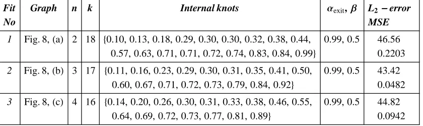
Table 1. Summary of test functions.

Function Specification

1 f1HxL=ÅÅÅÅÅÅÅÅÅÅÅÅÅÅÅÅÅÅÅÅÅ₁₊10₁₀₀x_x2 2 f2HxL=H4x-2L+2‰-16H4x-2L

2

3 f3HxL=sinH8x-4L+2‰-16H4x-2L

2

HeaviSine f4HxL=4 sinH4pxL-sgnHx-0.3L-sgnH0.72-xL

Doppler f5HxL=è!!!!!!!!!!!!!!!!!xH1-xLsinIÅÅÅÅÅÅÅÅÅÅÅÅÅÅÅÅÅÅÅÅ2p_HxH_+e1+e_LLM, e =0.05 Bumps f6HxL=‚

jhjI1+° x-sj

ÅÅÅÅÅÅÅÅÅÅÅÅ

wj •M

-4

, 8hj<=84, 5, 3, 4, 5, 4.2, 2.1, 4.3, 3.1, 5.1, 4.2<

8sj<=80.1, 0.13, 0.15, 0.23, 0.25, 0.40, 0.44, 0.65, 0.76, 0.78, 0.81<

8wj<=80.005, 0.005, 0.006, 0.01, 0.01, 0.03, 0.01, 0.01, 0.005, 0.008, 0.005<

Blocks f7HxL=‚

jhj

1+sgnHx-sjL

ÅÅÅÅÅÅÅÅÅÅÅÅÅÅÅÅÅÅÅÅÅÅÅÅÅÅÅÅÅ₂ , 8hj<=84,-5, 3,-4, 5,-4.2, 2.1, 4.3,-3.1, 2.1,-4.2<

8sj<=80.1, 0.13, 0.15, 0.23, 0.25, 0.40, 0.44, 0.65, 0.76, 0.78, 0.81<

The data sets, used to test GeDS were simulated by adding noise to each of the seven functions, as given in Table 1. As seen, we have included examples testing GeDS for different values of SNR, and for various characteristics of the data set: small and large sample sizes, x-values in a grid or uniformly generated within different intervals

xœ@a,bD. In all examples, the noise has a Normal distribution, with the exception of Example 1, where the noise is uniformly distributed. Note also that the test functions included in Table 2 possess different smoothness properties: some of them are relatively smooth, others very wiggly.

Table 2. Summary of examples used to test GeDS.

Example No

Function

HdataL

Interval Sample size, N

Data

xi, i=1, ..., N

Noice level,

se

SNR

1 f1HxL @-2, 2D 90 xi= -2+ÅÅÅÅÅÅÅÅÅÅÅÅÅÅÅÅÅÅÅÅH2-₈₉H-2LL Hi-1L UH-0.05, 0.05L

-2 f2HxL @0, 1D 256 150

UH0, 1L 0.6, 0.4, 0.25 0.25

2, 3, 5 5

3 f3HxL @0, 1D 256 UH0, 1L 0.3 3

4 HeaviSine @0, 1D 2048 xi= ÅÅÅÅÅÅÅÅÅÅÅÅ₂₀₄₇1 Hi-1L 1 7

5 Doppler @0, 1D 2048 xi= ÅÅÅÅÅÅÅÅÅÅÅÅ₂₀₄₇1 Hi-1L 1 7

6 Bumps @0, 1D 2048 xi= ÅÅÅÅÅÅÅÅÅÅÅÅ₂₀₄₇1 Hi-1L 1 7

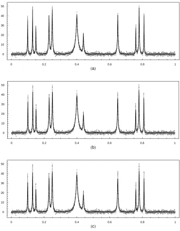
7 Blocks @0, 1D 2048 xi= ÅÅÅÅÅÅÅÅÅÅÅÅ₂₀₄₇1 Hi-1L 1 7

8 Titanium

Heat Data

@595, 1075D 49 xi=595+10Hi-1L -

MSE=i k jjjjj‚

i=1 N

IfHxiL- f

`

Dk,nHxiLM

2y

{ zzzzzìN.

Note that, in practice, the underlying function is unknown and a set of observations is fitted. For this reason, we give also the L2-error of approximation, defined as è!!!!!!!!!RSS .

However, for fair comparison between the smoothing methods, one would need all model parameter values, such as, number of knots (regression functions) and degree of the spline fits etc., which often are not reported in full. The Titanium Heat Data example is appropriate to compare different smoothing methods since the data are real and DeBoor and others have published the number and position of the knots and the degree of their spline fits. For fair comparison of the speed of computation one would need to implement all available methods using the same hardware and software, and test them on entirely identical simulated data sets. Such a comparison is outside the scope of this paper.

We have run GeDS with 400 simulated data sets for Examples 1-3 and 31 data sets for Examples 4-7. This allows us to compute the median of the MSE, obtained using GeDS, and compare it with the MSE medians given by other authors. However, in order to illustrate how GeDS performs, in each example we have used a single data set randomly chosen among the simulated data sets.

We compare most of our results, except those for the Blocks and Bumps examples, with the results of Luo and Wahba (1997) since, along with the median MSE values for their fits, they give also the order and the number of the basis functions. We have excluded the Bumps and Blocks since Luo and Wahba (1997) use versions of these functions which differ from ours, i.e., from those proposed by Donoho and Johnstone (1994).

Example 1. We start by testing GeDS on recovering the function f1, which appears in

-2 -1 0 1 2 HgL

-0.6 -0.4 -0.2 0 0.2 0.4 0.6

D6,2=81.1,-0.33,-0.12, 0.05, 0.12, 0.32<

-2 -1 0 1 2 HhL

-0.6 -0.4 -0.2 0 0.2 0.4 0.6

D7,2=8-1.1,-0.33,-0.12, 0.05, 0.12, 0.32, 0.96<

-2 -1 0 1 2 HeL

-0.6 -0.4 -0.2 0 0.2 0.4 0.6

D4,2=8-0.33,-0.12, 0.12, 0.32<

-2 -1 0 1 2 HfL

-0.6 -0.4 -0.2 0 0.2 0.4 0.6

D5,2=8-1.1,-0.33,-0.12, 0.12, 0.32<

-2 -1 0 1 2 HcL

-0.6 -0.4 -0.2 0 0.2 0.4 0.6

D2,2=8-0.33, 0.32<

-2 -1 0 1 2 HdL

-0.6 -0.4 -0.2 0 0.2 0.4 0.6

D3,2=8-0.33, 0.12, 0.32<

-2 -1 0 1 2 HaL

-0.6 -0.4 -0.2 0 0.2 0.4 0.6

D0,2=8<

-2 -1 0 1 2 HbL

-0.6 -0.4 -0.2 0 0.2 0.4 0.6

D1,2=80.32<

-2 -1 0 1 2 HeL

-0.6 -0.4 -0.2 0 0.2 0.4 0.6

-2 -1 0 1 2 HfL

-0.6 -0.4 -0.2 0 0.2 0.4 0.6

-2 -1 0 1 2 HcL

-0.6 -0.4 -0.2 0 0.2 0.4 0.6

-2 -1 0 1 2 HdL

-0.6 -0.4 -0.2 0 0.2 0.4 0.6

-2 -1 0 1 2 HaL

-0.6 -0.4 -0.2 0 0.2 0.4 0.6

D8,2=8-1.1,-0.33,-0.12,-0.05, 0.05, 0.12, 0.32, 0.96<

-2 -1 0 1 2 HbL

-0.6 -0.4 -0.2 0 0.2 0.4 0.6

Fig. 5. (Example 1) Graphs of the final B-spline fits, produced by GeDS: (a) linear; (b) and (e) quadratic, correspondingly without and with its control poly-gon; (c) and (f) cubic, correspondingly without and with its control polypoly-gon; (d) the control polygons of the fits in (a) - the thick line, in (b) - the dashed line and in (c) - the dotted line; The dotted function in (a), (b), (c) is the true function.

The details of the final linear, and its corresponding quadratic and cubic spline fits for Example 1 are presented in Table 3. Note that the values for aexit and b are the

"automatic" preassigned values 0.9, 0.5. As can be seen, the function f1 is symmetric

with median number of regression functions n+k =10, have median L2-errors

corre-spondingly 0.26, 0.267, 0.264, which are lower than 0.277, obtained by Schwetlick and Schütze (1995) for a quartic fit with the same number of regression parameters and optimally located knots. For all 400 linear fits, the number of internal knots used by GeDS is 8 or 9. Let us note that the computation time for the fits given in Table 3 is less then a second (0.89 sec.) and does not involve any complicated search procedures. We have produced also a quartic GeDS fit which has five internal knots as does the optimal quartic fit of Schwetlick and Schütze (1995), obtained starting from fifteen knots and after three time consuming knot generation, removal and relocation stages. Our quartic fit has L2-error equal to 0.46 which indicates that it does not deviate considerably from

the (locally) optimal solution.

Table 3. (Example 1) The linear, and its corresponding quadratic and cubic fits produced by GeDS .

Fit No

Graph n k Internal knots aexit, b L2-error, MSE 1 Fig. 5,HaL 2 8 8-1.1,-0.33,-0.12,-0.05, 0.05, 0.12, 0.32, 0.96< 0.9, 0.5 0.2699, 0.000189

2 Fig. 5,HbL 3 7 8-0.69,-0.22,-0.09, 0.00, 0.09, 0.22, 0.64< 0.9, 0.5 0.2944, 0.000127

3 Fig. 5,HcL 4 6 8-0.51,-0.17,-0.04, 0.04, 0.16, 0.47< 0.9, 0.5 0.2631, 0.000119

Example 2. This smooth function first appears as a test example in Fan and Gijbels (1995). It has been used later by Luo and Wahba (1997), Denison at al. (1998) and Zhou and Shen (2001) to test their fitting procedures. With this example, we illustrate that our algorithm works well for data sets with different sample sizes and various noise levels, assuming e is normally distributed. It takes between 0.89 sec and 1.66 sec to compute the GeDS fits, given in Table 4. The L2-errors of all the fits are within the noise level

and their visual quality is very good, as can be seen from Fig. 6. The median MSE value of the 400 linear fits, for se =0.4, with median number of internal knots k =5, is 0.009.

This is lower than the MSE value 0.012 of Luo and Wahba (1997), and is equal to that of Zhou and Shen (2001), both obtained using cubic splines with higher number of regression functions (e.g., 13 for the fit of Luo and Wahba (1997)). Let us note that for all 400 linear fits the number of internal knots used by GeDS is between 4 and 6. The linear and cubic fits corresponding to the quadratic fit No 3, Table 4, have five and three internal knots and 0.0066 and 0.0277 MSE values respectively.

Table 4. (Example 2) Summary of fits produced by GeDS.

Fit No

Graph N se n k Internal knots aexit,b L2-error, MSE 1 Fig. 6,HaL 150 0.25 3 4 80.37, 0.46, 0.54, 0.62< 0.9, 0.5 2.87, 0.001282

2 Fig. 6,HbL 256 0.25 3 4 80.38, 0.46, 0.54, 0.63< 0.9, 0.5 4.01, 0.001359

3 Fig. 6,HcL 256 0.4 3 4 80.38, 0.46, 0.54, 0.60< 0.95, 0.5 6.17, 0.006573

0 0.2 0.4 0.6 0.8 1 HcL

-3

-2

-1 0 1 2 3

0 0.2 0.4 0.6 0.8 1

HdL

-3

-2

-1 0 1 2 3

0 0.2 0.4 0.6 0.8 1

HaL

-3

-2

-1 0 1 2 3

0 0.2 0.4 0.6 0.8 1

HbL

-3

-2

-1 0 1 2 3

Fig. 6. (Example 2) Graphs of the final quadratic B-spline fits, produced by GeDS: (a) N=150, s =0.25; (b) N=256, s =0.25; (c) N=256, s =0.4; (d)

N=256, s =0.6; The dotted function in (a), (b), (c), (d) is the true function.

Note that the first two fits in Table 4 are obtained with aexit=0.9 and b =0.5. Since the

noise levels for fits No 3 and 4 are higher than for fits No 1 and 2, aexit has been

increased to 0.95, because, in the case of a smooth function and a high noise level, the relative improvements in RSS from one step to another would be smaller and more steps would be needed to recover the function.

Example 3. The function f3 (see Table 1) appears as a test example in Fan and Gijbels

(1995), Luo and Wahba (1997), Denison at al. (1998) and Zhou and Shen (2001). Using the GeDS algorithm we have produced linear, quadratic and cubic fits whose details are given in Table 5. The SNR of the sample data is 3, as for fit No 3 of Example 2. Since

f3 is also relatively smooth we have used aexit=0.95 and b =0.5 in order to obtain the

fits in Fig. 7 (e) and (f), which have very good visual quality and low MSE values. The GeD spline fits No 1-3 of Table 5, which have the same number of regression functions

k+n, are obtained with the preassigned "automatic" values aexit=0.9 and b =0.5. As

seen from Fig. 7 (a), (c) and (d), the linear and quadratic fits are sufficiently accurate while the cubic one underfits the data. Adding one more knot by running GeDS with the higher value of aexit=0.95 improves the cubic fit as illustrated by Fig. 7 (f). The

behav-ior of the stopping rule is illustrated in Fig.7 (b). It can be seen that with aexit=0.9 the

means that the MSE of the linear fit with 8 knots is at least 90% of the value 0.082677, i.e., the MSE has stabilized for three consecutive steps at which models with 6, 7 and 8 knots have been computed. If aexit=0.95 the algorithm exits one step later, with 7

internal knots for the linear fit and RSSêN =0.07967 since the improvement in RSSêN

for the next two consecutive steps is less than 5% of 0.07967. So, we see that our stop-ping rule, based on the idea of exiting upon reaching a certain level of stabilization in MSE, selects models with the appropriate number of knots.

0 0.2 0.4 0.6 0.8 1

HeL

-1 0 1 2 3

0 0.2 0.4 0.6 0.8 1

HfL

-1 0 1 2 3

0 0.2 0.4 0.6 0.8 1

HcL

-1 0 1 2 3

0 0.2 0.4 0.6 0.8 1

HdL

-1 0 1 2 3

0 0.2 0.4 0.6 0.8 1

HaL

-1 0 1 2 3

0 1 2 3 4 5 6 7 8 9

Number of knots HbL

0.2 0.4 0.6 0.8 1

E

S

M a

aexit=0.9

aexit=0.95