A Comparison of Forecasting Procedures for Macroeconomic Series : The Contribution of Structural Break Models

S

TRATHCLYDE

D

ISCUSSION

P

APERS IN

E

CONOMICS

D

EPARTMENT OF

E

CONOMICS

U

NIVERSITY OF

S

TRATHCLYDE

G

LASGOW

A COMPARISON OF FORECASTING PROCEDURES FOR

MACROECONOMIC SERIES: THE CONTRIBUTION OF

STRUCTURAL BREAK MODELS

B

Y

LUC

BAUWENS,

GARY

KOOP,

DIMITRIS

KOROBILIS

AND

JEROEN

V.K.

ROMBOUTS

A COMPARISON OF FORECASTING PROCEDURES FOR

MACROECONOMIC SERIES: THE CONTRIBUTION OF

STRUCTURAL BREAK MODELS

Luc Bauwens, CORE Gary Koop, University of Strathclyde

Dimitris Korobilis, CORE, Jeroen V.K. Rombouts, HEC Montreal and CORE

January 24, 2011

Abstract: This paper compares the forecasting performance of different models which

have been proposed for forecasting in the presence of structural breaks. These models differ

in their treatment of the break process, the parameters defining the model which applies in

each regime and the out-of-sample probability of a break occurring. In an extensive

empir-ical evaluation involving many important macroeconomic time series, we demonstrate the

presence of structural breaks and their importance for forecasting in the vast majority of

cases. However, we find no single forecasting model consistently works best in the presence

of structural breaks. In many cases, the formal modeling of the break process is important

in achieving good forecast performance. However, there are also many cases where simple,

rolling OLS forecasts perform well.

Keywords: Forecasting, change-points, Markov switching, Bayesian inference.

JEL Classification: C11, C22, C53.

Acknowledgements: This research was supported by the ESRC under grant

RES-062-23-2646, and by the contract ”Projet d’Actions de Recherche Concert´ees” 07/12-002 of the

”Communaut´e francaise de Belgique”, granted by the ”Acad´emie universitaire Louvain”. This

text presents research results of the Belgian Program on Interuniversity Poles of Attraction

1

Introduction

Structural breaks are commonly found to be present in many macroeconomic and financial

time series (e.g. Stock and Watson (1996) and Ang and Bekaert (2002)) and to be one

of the major reasons of poor forecasting performance (e.g. Clements and Hendry (1998)).

This has led to several papers which work with forecasting methods which are robust to

breaks (e.g. Pesaran and Timmermann (2007), Eklund, Kapetanios, and Price (2009) or

Clark and McCracken (2009)) or formally model the break process (e.g. Pesaran, Pettenuzzo,

and Timmermann (2006), Koop and Potter (2007), Giordani and Kohn (2008), Maheu and

Gordon (2008) and D’Agostino, Gambetti, and Giannone (2009)). It is an open empirical

question as to which types of methods or models will work best when dealing with the sort

of structural change present in many macroeconomic data sets. The purpose of this paper

is to shed light on this question. We compare empirically the forecasting performance of

existing models that explicitly allow for structural breaks both in the sample period and in

the forecast period. Two such models are given in Pesaran, Pettenuzzo, and Timmermann

(2006), hereafter PPT, and Koop and Potter (2007), hereafter KP, and these form the main

focus of our forecasting evaluation.1

Conventional time-varying parameter (TVP) models such

as that used by D’Agostino, Gambetti, and Giannone (2009) also allow explicitly for structural

breaks in-sample and out-of-sample and are also included in our forecasting evaluation. In

addition, we include some benchmark forecasting procedures such as recursive and rolling

OLS.

Our study is in the spirit of Meese and Geweke (1984), Stock and Watson (1996) and

Mar-cellino, Stock, and Watson (2006) in the sense that we investigate the performance of various

forecasting approaches at different forecast horizons in a set of macroeconomic time series

using relatively simple forecasting models (i.e. extensions of autoregressive, AR, models).

We evaluate forecast performance using a variety of metrics. In addition to a conventional

measure based on point forecasts (i.e. root mean squared forecast error, RMSE), we

com-pare the approaches using average predictive likelihoods (APL) which are based on the entire

predictive density.

1_{The mixture innovation model of Giordani and Kohn (2008) can also be used to forecast in the presence}

In this paper we focus on PPT and KP as two representative examples of models which

address the issues which arise when forecasting subject to structural breaks. Such forecasting

models can differ in three important aspects. First, they can differ in the priors they use for

the parameters which define the conditional mean (and possibly the conditional variance) of

the dependent variable. PPT uses a hierarchical prior of the sort commonly used in the panel

data literature where conditional mean coefficients are all assumed to be drawn from some

common distribution. KP uses a hierarchical prior motivated by the state space literature

where the conditional mean coefficients in the most recent regime are most relevant when a

break occurs. Second, they can differ in the hierarchical prior used for the regime durations.

For instance, PPT assume a Geometric distribution for regime duration whereas KP assume

a Poisson distribution. Third, they can differ in whether they impose the restriction that a

precise number of breaks occurs in a sample of size T or whether the number of in-sample

breaks is treated as unknown. The former approach is adopted by PPT, involves an (arguably,

see Koop and Potter (2007) and Koop and Potter (2009)) unattractive prior at the end of the

sample and requires the calculation of marginal likelihoods. The latter approach is adopted

by KP and does not involve these drawbacks.

Of course, it is an empirical matter which of these approaches works well in practice and

it is possible that each approach works well in some cases but not others. KP and PPT each

illustrate the performance of their approaches with a single time series (and with modeling

details calibrated to that particular series). The purpose of this paper is to investigate these

and related approaches for a wide variety of macroeconomic series. We select twenty-three

of the most important quarterly US macroeconomic time series and compare PPT and KP

to a variety of forecasting methods. We find that structural breaks are an important feature

of most of the time series we consider. Handling such breaks is shown to be an important

issue for forecasting. However, we find that there is no one single method which can be

recommended universally. That is, for some series PPT forecasts best, for others KP does,

for others simpler methods such as rolling OLS forecasts performs best. We argue that this is

empirically-sensible and stress the importance of tailoring forecasting models to the empirical

KP models that we use in our empirical evaluation. Technical details are provided in

ap-pendices. In Section 3, we present the estimation results of applying PPT and KP to the

series we analyze, focussing on what breaks we find in the series. In Section 4 we discuss the

implementation of our forecasting evaluation and in Section 5 we present our main results.

Section 6 contains the results of sensitivity analyses and the last section our conclusions.

2

Models with Structural Breaks

In this section, we present and compare the PPT and KP models. After providing a framework

for structural break models (sub-section 2.1), we discuss how the parameters of different

regimes are linked (sub-section 2.2), how the break process is modelled (sub-section 2.3), and

how the number of breaks is determined (sub-section 2.4).

2.1 A Framework for Structural Break Modelling

A linear regression model framework for discussing structural break models is:

yt=Ztβst +σstεt, (1)

where yt is the dependent variable,Zt (with m elements in total) contains lagged dependent

variables or lagged exogenous variables available for forecastingyt, and εtis i.i.d. N(0,1).

Equation (1) allows forβst andσst to vary over time withst∈ {1, .., K}a random variable

indicating which regime applies at time t. The vector βst determines the conditional mean

of yt and, thus, we will refer to them as conditional mean coefficients with σst being the

volatilities.

Different structural break models vary in the way they model the break process. To

simplify the exposition, we will focus here on βst and assume σst = σ. But we stress that

breaks in volatilities can be modelled in exactly the same manner as breaks in the conditional

mean coefficients and in our empirical work we allow for breaks in volatility.2

Suppose we are working with a model withK−1 breaks which occur at unknown times

2_{Furthermore, we could allow for breaks in volatility to occur independently of breaks in the conditional}

mean. In this case, st is a bivariate discrete random variable with the first element controlling breaks in

τ1, .., τK−1. Thus, we can write:

yt= 

         

         

Ztβ1+σεt ifst= 1 (i.e. t≤τ1),

Ztβ2+σεt ifst= 2 (i.e. τ1< t≤τ2),

...

ZtβK−1+σεt ifst=K−1 (i.e. τK−2< t≤τK−1),

ZtβK+σεt ifst=K (i.e. τK−1 < t≤T).

(2)

Different structural break models arise through different formulations forβst andst. From

a Bayesian point of view these can be interpreted as hierarchical priors. In the next two

sections, we discuss modelling of βst and strespectively.

2.2 Linking the Conditional Mean Coefficients in Different Regimes

It is possible to allow for βj for j = 1, .., K to be completely independent of one another

(i.e. after a break occurs, pre-break information provides absolutely no information about

what likely values for the new conditional mean coefficients are). But, in practice, it is

typically desirable to avoid such independence. Even when simply doing an in-sample analysis,

structural break models can be over-parameterized and placing more structure on the model

can help avoid this problem. That is, if βj is completely independent of all other regimes,

one must estimate it using data only from regime j. With relatively short macroeconomic

data sets, possibly high dimensional βj and possibly multiple structural breaks, it may be

hard to obtain precise estimates of βj. When forecasting subject to structural breaks, an

even more serious problem occurs. Suppose a break occurs during the forecast period, and

the conditional mean coefficient switches from βj to βj+1. Forecasting must be done using

βj+1. If we assume complete independence of conditional mean coefficients across regimes,

then immediately after the break we have no data-based information to estimate βj+1. In a

Bayesian forecasting exercise, this means the prior forβj+1 will be used to produce forecasts.

Given a common desire to use relatively noninformative priors, this could lead to extreme

and unreasonable forecasts when a break occurs. This has motivated various models which

linkβj and βj+1 in some manner.

form:

βj =β0+uj

for j= 1, .., K, whereuj is i.i.d. Nm(0, B0) or, equivalently, in Bayesian language, a

hierar-chical prior of the form:

βj ∼Nm(β0, B0), (3)

the parameters β0 andB0 are assumed unknown and can be estimated from the data. Thus,

the conditional mean coefficients in each regime are drawn from a common distribution. This

practice is commonly used in panel data models with random effects or in random coefficient

models and results from that literature can easily be adapted to show that β0 andB0 reflect

average values across all regimes. If a break occurs in a forecast period, this means that the

new value of the conditional mean coefficients will be drawn from a distribution which reflects

the values of the coefficients from all past regimes. This is an empirically sensible approach

in environments where breaks occur, but in a recurrent way. It allows, for instance, for the

1950s, 1970s, 1990s and 2000’s to be different regimes, but the regime in the 2000s is just as

likely to be similar to the 1950s as to more recent regimes.

In contrast, KP adopt a hierarchical prior motivated by the state space literature on TVP

models. They specify random walk evolution of coefficients:

βj =βj−1+uj

where uj is specified as above, or equivalently,

βj|βj−1 ∼Nm(βj−1, B0). (4)

The KP prior is similar to the PPT prior, except that, when a structural break occurs, the

conditional mean coefficients are drawn from a distribution centered at βj−1. Thus, it is the

most recent regime which has the most influence on conditional mean coefficients in a new

regime. This is a common modelling assumption in macroeconomic models such as

TVP-VARs and, indeed, the KP model is equivalent to a TVP regression model if st=tand, thus,

K =T.

It is worth noting that with either the PPT prior or the KP prior, it is possible to introduce

exogenous explanatory variables into the hierarchical prior (e.g. in the PPT prior we could

have β0 =Wtb0 for some lagged variablesWt) although we do not explore this avenue in the

2.3 Modeling the Break Process

The break process is modelled throughST = (s1, .., sT)′ wherest∈ {1,2, .., K}are the regime identifying (or state) variables defined previously. It is possible to use a noninformative prior

which does not restrict the timing of the breaks. This is an approach developed in Koop and

Potter (2009). However, unless the number of breaks is small, computation is difficult (or

infeasible) due to the large number of possible configurations ofK breakpoints. Furthermore,

when forecasting under structural breaks, it is necessary to forecast the probability that a

break occurs during the forecast period and this cannot be done using a noninformative prior

forST. This has led to an interest in informative hierarchical priors for the break process.

The most popular of these is developed in Chib (1998) and adopted by PPT. This begins by

assuming a restricted Markov process forST:

Pr (st=i|st−1=i) =pi

Pr (st=i+ 1|st−1 =i) = 1−pi.

(5)

Thus, if regimeiholds at timet−1, then at timet the process can either remain in regimei

(with probabilitypi) or a break occurs and the process moves to regimei+ 1 (with probability

1−pi).

Equation (5) can be interpreted as a hierarchical prior. Note that the durations of regimes

are defined as:

di=τi−τi−1

and it can be shown that (5) implies a Geometric prior distribution fordi. KP argue that this

may be restrictive in some situations. For instance, the geometric distribution is decreasing

and, thus, this hierarchical prior imposesp(di)> p(di+ 1). They suggest the use of the more

flexible Poisson distribution for the durations:

di−1∼P o(λi) (6)

whereP o(λi) denotes the Poisson distribution with meanλi. However, in the present paper,

in order to maintain a fair degree of computational simplicity and comparability across our

forecasting approaches, we implement the KP approach using the Geometric prior implied by

Either of these two hierarchical priors can be used for forecasting purposes. However,

when forecasting with structural breaks, we need to estimate the probability that a break

occurs during the forecasting period. In some cases, it can be desirable to include more

information on the break process or further restrict the model to ensure parsimony. Thus, we

note a few empirically useful extensions of the previous priors. First, it is possible to assume

a hierarchical prior forpi orλisuch that they are drawn from some common distribution. An

extreme limiting case of such an approach would involve settingλ1 =...=λKorp1=...=pK.

Second, it is possible to allow for either pi or λi to depend on lags of themselves (e.g. the

prior forλi can depend onλi−1) or durations of past regimes. Some of these possibilities are

investigated in KP, but are not pursued here.

2.4 Choosing the Number of Breaks

Thus far, we have said nothing about choosing K−1, the number of breaks. But this raises an important issue. Note that both the Geometric and Poisson duration distributions which

arise using (5) or (6) are unbounded distributions. Thus, it is possible that any regime endures

beyond the end of the sample. For instance, if the sample runs from t= 1, .., T and the model

has three breaks, it is possible that sT = 1 or 2 and, thus, that the third regime has not

begun beforeT. PPT and KP adopt two different ways of dealing with this issue, which we

describe in turn.

PPT, following Chib (1998), impose additional prior information beyond (5). Intuitively,

we can impose that exactly K regimes occur in sample by adding prior information of the

form:

Pr[sT =K|sT−1=K] = Pr[sT =K|sT−1=K−1] = 1. (7)

Thus, if the process reaches the final regime before the end of the sample it stays there. But

if it has not reached the final regime by period T −1, it must switch to the final regime. If K exceeds 2, additional restrictions are required. To express these restrictions in words,

consider the case K = 3. If, in period T−1, we are not already in the third regime, then it must be the case that a regime switch occurs in period T and this must be imposed on the

the end of the sample, leading to a prior which is quite informative (and, thus, potentially

influential) precisely at the time forecasting is being done.

KP simply recommend working with models which allow for breakpoints to occur

out-of-sample. Statistically, working with such models poses no difficulties for a Bayesian using a

proper prior. Consider the case where regimejoccurs entirely out-of-sample. It appears that

there is no data to directly estimate βj. However, Bayesian inference is still possible. If the

prior forβj were independent of the conditional mean coefficients in the other regimes, then

its posterior would simply equal its prior. Such an approach would allow for valid statistical

inference but could yield poor forecasting results unless strong prior information existed about

βj. However, using hierarchical priors such as (3) or (4) allows for data information from

in-sample regimes to spill over into out-of-in-sample regimes and, thus, the posterior for βj will

contain data information. More importantly, allowing for regimes to occur out-of-sample

allows the researcher to estimate the number of regimes in-sample. For instance, if the

researcher allows for two breakpoints, but one of these occurs after timeT, then (in-sample)

this is equivalent to estimating a model with one breakpoint. This means that the researcher

can simply select a value for the maximum number of breakpoints to allow for as opposed

to doing a search over all possible numbers. By contrast, with the PPT approach, marginal

likelihoods are calculated forK= 1, ..Kmax

and the value with the highest marginal likelihood

is selected. This need for calculation of marginal likelihoods increases the computational

burden.

3

Breaks in US Macroeconomic Series

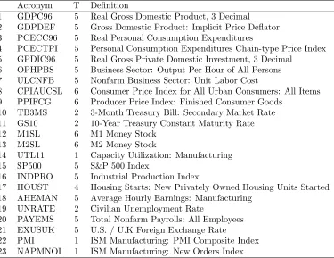
We apply the PPT and KP models to twenty-three quarterly series for the USA (listed in Table

1) which are among the most important macroeconomic variables. The sample period is 1959,

first quarter, till 2010, second quarter. As indicated in the table, we have transformed most

series to growth rates or first differences, and in this we are proceeding as in the literature,

see e.g. Stock and Watson (1996). We use AR(q) models in each regime, hence, Zt in (2)

contains an intercept and the first q lags of yt.

Details about prior densities and posterior evaluation are provided in Appendix A for PPT

models and in Appendix B for KP. Further discussion of the prior is given in Section 6.2.

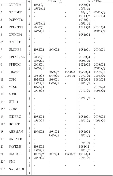
In Table 2 we report the break dates found in the PPT-AR(1) and AR(4) models (called

PPT1 and PPT4 hereafter), and similarly KP-AR(1) and AR(4) models (KP1 and KP4),

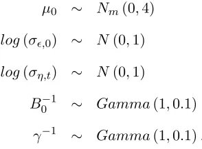
using the complete sample. In Table 3 we report the posterior means of the AR(1) equations

for each regime. The reported break dates are medians of posterior distributions and there is

some uncertainty (though not much) about these point estimates.

We do not find any break in six series (6, 14, 15, 17, 22, 23) both with PPT and KP

(irrespective of the lag order), and in four other series with PPT (series 2, 5, 13, 19), see

Table 2. No series has more than two breaks with KP, while only series 21 has three breaks

with PPT1. To a large extent, the break numbers and dates are robust with respect to the

lag order (1 or 4), keeping in mind that for dates we report posterior medians. This is much

less the case with respect to the type of model (PPT and KP). For example, even if three

series (4, 8, 9) have a break in the last three years of the sample according to both models,

KP detects more breaks of this type than PPT, see series 2, 12, and 16.

Thus there is evidence that macroeconomic series are subject to breaks since about three

quarters of our series have at least one break when modeled by structural break models. The

next obvious question is how large are the parameter changes when breaks occur and what

parameters are affected. Table 3 contains the posterior means of the parameters of the AR(1)

equations of each regime for each series, over the full sample period. Focusing on the series

with more than one regime (for PPT and KP), we observe that the most sensitive parameter

is the variance of the error term. It decreases substantially for some series in the first half

of the eighties, see the break in series 1, 7, 16, 18, and 20 with both models, and in series 5

with KP, corresponding to what has been named the great moderation (the decrease is about

seventy-five percent on average for these series). The error variance increases quite a lot in

2007 or 2008 for series 4, 8, 9 with PPT, and 2, 8, 9 and 16 with KP (see the last break).

These increases correspond to the great recession triggered by a widespread financial crisis.

Other cases are the reduction by half of the variance of series 3 in 1993, and the quadrupling

for series 7 in 2000. The interest rate series (10 and 11) witness also large changes: a tenfold

increase in 1979 corresponds to the beginning of the Volcker period at the Fed, which is

Table 1: Variables used in forecast evaluation

Acronym T Definition

1 GDPC96 5 Real Gross Domestic Product, 3 Decimal 2 GDPDEF 5 Gross Domestic Product: Implicit Price Deflator 3 PCECC96 5 Real Personal Consumption Expenditures

4 PCECTPI 5 Personal Consumption Expenditures Chain-type Price Index 5 GPDIC96 5 Real Gross Private Domestic Investment, 3 Decimal

6 OPHPBS 5 Business Sector: Output Per Hour of All Persons 7 ULCNFB 5 Nonfarm Business Sector: Unit Labor Cost

8 CPIAUCSL 6 Consumer Price Index for All Urban Consumers: All Items 9 PPIFCG 6 Producer Price Index: Finished Consumer Goods

10 TB3MS 2 3-Month Treasury Bill: Secondary Market Rate 11 GS10 2 10-Year Treasury Constant Maturity Rate

12 M1SL 6 M1 Money Stock

13 M2SL 6 M2 Money Stock

14 UTL11 1 Capacity Utilization: Manufacturing 15 SP500 5 S&P 500 Index

16 INDPRO 5 Industrial Production Index

17 HOUST 4 Housing Starts: New Privately Owned Housing Units Started 18 AHEMAN 5 Average Hourly Earnings: Manufacturing

19 UNRATE 2 Civilian Unemployment Rate

20 PAYEMS 5 Total Nonfarm Payrolls: All Employees 21 EXUSUK 5 U.S. / U.K Foreign Exchange Rate

22 PMI 1 ISM Manufacturing: PMI Composite Index

23 NAPMNOI 1 ISM Manufacturing: New Orders Index

T (transformation applied to original series): 1 = no transformation, 2 = first differ-ence, 4 = log, 5 = first difference of logged variables, 6 = second difference of logged variables. Sample period (after data transformation): 1959Q1-2010Q2 (206 observa-tions). Data source: St. Louis ALFRED database (http://alfred.stlouisfed.org).

In some series, the constant and the AR(1) coefficients change also, but less spectacularly

than the variance. This happens to the two interest rates. Keeping in mind that they are in

first differences, the changes of the coefficients (in particular the sign change of the constant)

around 1985 correspond to the start of a long period of decrease of interest rates. A change

of sign of the constant happens also in series 21 in the last quarter of 1967 (first break with

KP, second break with PPT). The British pound sterling came under pressure in the

mid-sixties since the exchange rate against the dollar was considered too high and was eventually

devalued by 14.3% to 2.40 on 18 November 1967. This suggests that the first break detected

Table 2: Break dates based on full sample

q PPT-AR(q) KP-AR(q)

1 GDPC96 1 1983:Q1 - - 1983:Q4

-4 1982:Q2 - - 1983:Q4

-2 GDPDEF 1 - - - 1984:Q3 2008:Q4

4 - - - 1981:Q2 2008:Q4

3 PCECC96 1 - - - 1993:Q1

-4 1987:Q2 - - 1992:Q2

-4 PCECTPI 1 2008Q1 - - 1991:Q3 2006:Q4

4 2007Q3 - - - 2008:Q4

5 GPDIC96 1 - - - 1984:Q4

-4 - - - -

-6∗ _{OPHPBS 1 - - - -}

-4 - - - -

-7 ULCNFB 1 1983Q2 1999Q2 - 1984:Q1 2000:Q1

4 - - - -

-8 CPIAUCSL 1 2008Q1 - - 2008:Q4

-4 2007Q3 - - 2008:Q4

-9 PPIFCG 1 2008Q1 - - 1972:Q3 2008:Q4

4 2007Q3 - - - 2008:Q4

10 TB3MS 1 - 1979Q2 1984Q3 1979:Q4 1985:Q1

4 1965Q1 1978Q3 1983Q4 1979:Q4 1985:Q2

11 GS10 1 1979Q2 1986Q1 - 1979:Q4 1986:Q4

4 1978Q3 1985Q2 - 1966:Q2

-12 M1SL 1 1978Q4 - - - 2008:Q3

4 1978Q1 - - 1979.Q2 2008:Q4

13 M2SL 1 - - - -

-4 - - - 1979.Q2

-14∗ _{UTL11 1 - - - -}

-4 - - - -

-15∗ _{SP500 1 - - - -}

-4 - - - -

-16 INDPRO 1 1982Q4 - - 1984:Q1 2008:Q2

4 1980Q3 - - 1983:Q4 2008:Q3

17∗ _{HOUST 1 - - - -}

-4 - - - -

-18 AHEMAN 1 1969Q2 1981Q4 - 1982:Q4

-4 1980Q2 - 1983:Q4

-19 UNRATE 1 - - - -

-4 - - - 1983:Q4

-20 PAYEMS 1 1983Q3 - - 1984Q2

-4 1982Q2 - - 1983:Q3

-21 EXUSUK 1 1967Q2 1967Q4 1971Q2 1967:Q4

-4 1966Q3 - - 1983:Q3

-22∗ _{PMI 1 - - - -}

-4 - - - -

-23∗ _{NAPMNOI 1 - - - -}

-4 - - - -

Table 3: Posterior means of AR(1) break models

S R PPT-AR(1) KP-AR(1) AR(1) full sample AR(1) last 40 data

c φ σ2 c φ σ2 c φ σ2 c φ σ2

1 1 0.55 0.30 1.12 0.62 0.28 1.10 0.52 0.32 0.69 0.19 0.49 0.36 2 0.39 0.46 0.32 0.38 0.45 0.29 - - - 0.51 0.29 0.26 2 1 0.12 0.87 0.09 0.14 0.87 0.10 0.11 0.87 0.09 0.33 0.41 0.09 2 - - - 0.24 0.35 0.04 - - - 0.29 0.58 0.03 3 - - - 0.23 -0.19 0.35 - - - -3 1 0.56 0.31 0.46 0.65 0.26 0.51 0.56 0.31 0.45 0.23 0.54 0.20

2 - - - 0.46 0.42 0.22 - - - 0.72 0.02 0.35 4 1 0.13 0.86 0.10 0.13 0.87 0.10 0.15 0.83 0.13 0.42 0.24 0.23 2 0.14 0.51 0.84 -0.09 0.01 0.64 - - - 0.40 0.49 0.08 3 - - - 0.20 0.10 0.45 - - - -5 1 0.07 0.18 0.21 0.10 0.10 0.30 0.07 0.18 0.21 -0.02 0.54 0.12

2 - - - 0.06 0.30 0.11 - - - 0.08 0.02 0.11 6∗ _{1 0.56 -0.01 0.72 0.56 -0.01 0.71 0.57 -0.01 0.71 0.59 0.10 0.53}

- - - 0.33 0.14 0.41 7 1 0.60 0.40 1.28 0.60 0.43 1.21 0.51 0.32 1.11 0.26 -0.14 1.01 2 0.47 0.14 0.33 0.47 0.14 0.33 - - - 0.55 0.08 0.34 3 0.39 -0.07 1.33 0.38 -0.07 1.35 - - - -8 1 0.00 -0.29 0.18 0.01 -0.30 0.18 -0.00 -0.30 0.27 -0.01 -0.35 0.76

2 -0.03 -0.30 2.69 -0.17 -0.30 3.62 - - - 0.00 -0.35 0.18 9 1 0.02 -0.38 1.08 0.03 -0.45 0.40 0.02 -0.32 1.69 0.05 -0.27 5.13 2 0.03 -0.30 19.08 0.02 -0.38 1.32 - - - 0.00 -0.37 1.65 3 - - - -0.16 -0.23 21.71 - - - -10 1 0.04 0.36 0.32 0.03 0.33 0.31 -0.01 0.23 0.57 -0.06 0.61 0.19

2 -0.01 0.25 3.80 -0.00 0.19 3.45 - - - 0.01 0.67 0.13 3 -0.03 0.55 0.14 -0.03 0.56 0.14 - - - -11 1 0.04 0.22 0.08 0.03 0.21 0.06 -0.00 0.23 0.23 -0.06 0.02 0.13

2 0.01 0.22 0,93 -0.02 0.24 0.22 - - - -0.05 0.38 0.23 3 -0.04 0.22 0.16 -0.05 0.20 0.15 - - - -12 1 0.01 -0.18 0.36 -0.00 -0.32 0.77 0.00 -0.30 0.96 0.05 -0.28 2.12

2 -0.00 -0.31 1.35 -0.04 -0.24 7.30 - - - -0.07 -0.11 0.94 13 1 -0.00 -0.15 0.48 -0.01 -0.15 0.46 -0.01 -0.15 0.47 -0.04 -0.16 0.79

- - - -0.05 -0.12 0.30

14∗ _{1 0.25 0.97 0.02 0.26 0.97 0.02 0.25 0.97 0.02 0.42 0.94 0.02}

- - - 0.45 0.95 0.01 15∗ _{1 0.11 0.24 0.45 0.11 0.23 0.44 0.11 0.23 0.45 -0.04 0.36 0.67}

- - - 0.28 -0.15 0.50

16 1 0.39 0.44 4.00 0.46 0.45 3.11 0.35 0.51 1.99 -0.00 0.70 1.23 2 0.21 0.67 0.85 0.25 0.61 0.69 - - - 0.33 0.54 0.62 3 - - - 0.05 0.76 2.90 - - - -17∗ _{1 0.18 0.97 0.01 0.18 0.97 0.01 0.21 0.97 0.01 -0.27 1.03 0.01}

- - - 0.63 0.91 0.01 18 1 0.83 0.14 0.40 0.72 0.52 0.40 0.38 0.65 0.26 0.63 0.04 0.07 2 1.00 0.47 0.26 0.55 0.22 0.07 - - - 0.49 0.28 0.07 3 0.58 0.19 0.08 - - - -19 1 0.01 0.64 0.07 0.01 0.64 0.07 0.01 0.65 0.07 0.03 0.74 0.07

- - - -0.02 0.70 0.03

20 1 0.14 0.76 0.17 0.15 0.76 0.17 0.08 0.83 0.10 -0.02 0.86 0.07 2 0.03 0.89 0.04 0.03 0.90 0.04 - - - 0.06 0.88 0.03 21 1 -0.00 0.20 0.00 -0.00 0.19 0.00 -0.02 0.26 0.17 0.00 0.41 0.19 2 -0.31 0.27 0.40 -0.03 0.26 0.20 - - - 0.05 0.14 0.35 3 0.01 0.12 0.00 - - - -4 -0.03 0.24 0.22 - - - -22∗ _{1 0.89 0.83 0.16 0.96 0.82 0.15 1.01 0.81 0.15 0.93 0.82 0.13}

- - - 0.95 0.82 0.07 23∗ _{1 1.20 0.78 0.27 1.31 0.76 0.26 1.40 0.75 0.26 1.36 0.75 0.33}

- - - 1.30 0.77 0.14

S = series number (see Table 2); R = regime number. Each AR(1) is written yt =

c+φyt−1+σǫt. Two estimations are reported in the block ”AR(1) last 40 data”: on the

4

Forecasting Implementation

In this section, we explain how we forecast with the PPT and KP models, and in sub-section

4.3 we review briefly the other models with which we generate alternative forecasts to be

compared with the forecasts coming from the break models.

The setup is the following: we shall carry out a recursive forecasting exercise for the final

α percent of the observations. This means that we first estimate the models with an initial

sample consisting of 1−αpercent of the data, and we forecast future observations. Then we add one data point, estimate and forecast again, until we have consumed all the data.

4.1 Forecasting with PPT

With the PPT approach, if one were to assume that no breaks occur out-of-sample, forecasting

could be done in a straightforward way based on the posterior density of the the parameters

of the regime that holds at the end of the estimation sample. Such an approach, of course,

does not address the issue of forecasting when breaks can occur out-of-sample. Appendix A

provides details about how predictive simulation is implemented for the PPT model.

To choose the number of breaks, we choose a maximum number of regimes,Kmax

, evaluate

the marginal likelihood forK= 1, .., Kmax_{and select the optimal number of regimes as the one}

which maximizes the marginal likelihood. However, in the context of a recursive forecasting

exercise, we wantKmax_{to vary over time as the number of regimes can increase as time goes}

by. Accordingly, we adopt the following strategy.

Using the initial sample of observations, we calculate the optimal number of regimes as

described in the preceding paragraph. Then we begin our recursive forecasting exercise. Let

Kt be the number of regimes in a model using data through time t. We compute marginal

likelihoods for Kt = {1, . . . , Kt∗−1 + 1} where Kt∗−1 is the optimal number of regimes at

t−1 and select K∗

t as the value that maximizes the marginal likelihood. We do this for

t = T0+ 1, . . . , T −h where T0 = αT. Marginal likelihoods are calculated as described in

Bauwens and Rombouts (2010), based on output from the posterior simulator.

We calculate two predictive densities, one which assumes no future break, and one of

which allows for a possible single break in the forecast period. The necessary details are given

4.2 Forecasting with KP

With the KP approach, dealing with out-of-sample structural breaks is straightforward.

Suppose regime j holds at the end of the estimation sample (called t) and, thus, st = j.

The posterior simulation algorithm produces Pr (st+1=j|Yt) and Pr (st+1 =j+ 1|Yt), where

Yt = (y1, .., yt)′. Furthermore, the posterior simulation algorithm provides us with draws

from p(βj, σj|Yt) and p(βj+1, σj+1|Yt). These are the components needed to do

forecast-ing with structural breaks. Appendix C provides details about how predictive simulation is

implemented for the KP model.

Defining the optimal number of regimes for each sample in our recursive forecasting

exer-cise is done in a way similar to the PPT model described previously, but without the need to

compute marginal likelihoods. Using output from the posterior simulator using data through

time t, we calculate the optimal number of breaks as K∗

t = median(Pr(st|data)), i.e. the median of the posterior of the state variable of the last observation.

In particular, we run the model for t=T0 (where T0 =αT) for a large number of breaks.

Then instead of using marginal likelihoods to estimate the optimal number of breaks at time

T0, we just use the estimate K_T∗

0 =median(Pr(sT0|data)). In the next period (t=T0+ 1) we

estimate the KP model with KT0+1 breaks and forecast, where we define KT0+1 =K ∗

T0 + 1.

From the Gibbs sampler output we estimate K∗

T0+1 = median(Pr(sT0+1|data)). Then we

increase the observations by one (t=T0+ 2) and set KT0+2 =K ∗

T0+1+ 1 and so on.

In words, with number of observations t we always allow for one more break than the

optimal number of breaks estimated in the previous sample t−1. However, when we set the number of breaks using the formula Kt = Kt∗−1+ 1, this doesn’t necessarily mean that we

forecast with exactlyK_t∗₋1+ 1 breaks at timet. This is the maximum number of breaks. This

implies that it might be the caseK∗

t =Kt∗−1 so that the number of regimes we use to forecast

hasn’t changed. Therefore, as we progress at timet+ 1 we set Kt+1 =K_t∗+ 1 =K_t∗₋1 + 1.

Nevertheless, if the optimal number of estimated regimes at time t has actually changed to

K_t∗ = K_t∗₋1 + 1 (we discovered an additional break), then we ought to set at time t+ 1 a

maximum number of regimes Kt+1=K_t∗+ 1 =K_t∗₋1+ 2.

4.3 Forecasting with Other Approaches

In addition to the forecasting methods of KP and PPT outlined above, we consider a variety

of other ”no-break” models.

Our first approach is a standard TVP-AR(1) model. This is a restricted special case of

the KP approach. That is, if we adopt the KP framework but set st=t for all time periods

(or equivalently,Kmax

t =tand Pr (st=t|st−1 =t−1) = 1 then we obtain the standard TVP

model which is of the form

yt = Ztβt+σtεt

βt = βt−1+ut (8)

log(σt) = log(σt−1) +vt

whereεt∼N(0,1),ut∼N(0, B0) andvt∼N(0, δ). Note that for this special case we need extra care in defining our priors, since the autoregressive coefficients evolve as random walks

for allt periods and they can easily become explosive. The priors we use for this model are

β0 ∼ Nm(0,4Im)

log(σ0) ∼ N(0,1)

B0−1 ∼ W ishart m+ 1,(0.001 2

(m+ 1)R)−1

δ−1 ∼ Gamma(1,0.1).

whereR is a diagonal matrix with elements R{1,1} = 5 for the intercept, and R{i, i}= 1/i

for lag lengthi= 1, ..., p. Forecasting in this model requires first to simulate the future paths

of the time-varying coefficients βt and log(σt) using their random walk specifications. Then

conditional on these simulated out-of-sample coefficients, we forecast yT+h as in a simple

regression model.

We also present recursive and rolling AR(q) forecasting results (with q set to one and

to four). Bayesian inference is used for these models using the same prior density as in the

PPT implementations if we allow for only a single regime. For the rolling forecasts we use

a window of ten years (forty observations). We tried a window of five years but the forecast

results are much deteriorated by this choice. A window of ten years seems reasonable since

different enough from the sample used with the recursive approach.4

Finally we also use an unobserved component model with stochastic volatility (UC-SV).

We follow the formulation of Stock and Watson (2007), who specify a model with only a

time-varying trend (no AR dynamics), which takes the form

yt = µt+σǫ,tεt

µt = µt−1+ση,tηt (9)

log(σǫ,t) = log(σǫ,t−1) +vt

log(ση,t) = log(ση,t−1) +wt

where in this case, (εt, ηt)∼ N(0, I2), ut ∼N(0, γ1) and vt ∼N(0, γ2). For U.S. inflation,

Stock and Watson (2007) setγ1=γ2 = 0.2. We estimate these parameters and the priors we

use to forecast with this model are

µ0 ∼ Nm(0,4)

log(σǫ,0) ∼ N(0,1)

log(ση,t) ∼ N(0,1)

B0−1 ∼ Gamma(1,0.1)

γ−1 ∼ Gamma(1,0.1).

Forecasting in the above model is similar in spirit with the TVP and KP models. We first

need to simulate the future values of the time-varying parameters, and then plug in these

simulated values in the first equation in 9.

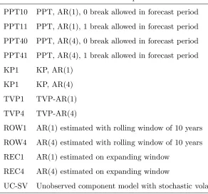
Table 4 lists the models used in the forecasting evaluations, with a short definition.

5

Results of Forecasting Evaluations

For each series listed in Table 1, we carry out a recursive forecasting exercise for the final thirty

percent of the observations: we first estimate the models with an initial sample consisting

of seventy percent of the data, and we forecast at the horizons h equal 1 and 4. Then we

Table 4: Models used in the forecasting evaluations

Name Description

PPT10 PPT, AR(1), 0 break allowed in forecast period

PPT11 PPT, AR(1), 1 break allowed in forecast period

PPT40 PPT, AR(4), 0 break allowed in forecast period

PPT41 PPT, AR(4), 1 break allowed in forecast period

KP1 KP, AR(1)

KP1 KP, AR(4)

TVP1 TVP-AR(1)

TVP4 TVP-AR(4)

ROW1 AR(1) estimated with rolling window of 10 years

ROW4 AR(4) estimated with rolling window of 10 years

REC1 AR(1) estimated on expanding window

REC4 AR(4) estimated on expanding window

UC-SV Unobserved component model with stochastic volatility

61 one-step and 58 four-step ahead forecasts on which we can base the forecast evaluations.

Forh > 1, our forecasts are all iterated (see, e.g., Marcellino, Stock, and Watson (2006) for

a motivation for use of iterated over direct forecasts).

Our forecast metrics are RMSE and the average of log predictive likelihoods (APL). RMSE

is based on point forecasts and we use the predictive median as point forecast. The predictive

likelihood is the predictive density evaluated at the observed outcome. This is estimated by

a nonparametric kernel smoother using draws from the predictive simulator.

For each series in Table 1, we provide in Appendix C the RMSE and APL values from the

recursive forecasting exercise. For one-step ahead forecasts, see Tables 13 (RMSE) and 15

(APL) and for four-step ahead forecasts see Tables 14 and 16. We report the relative values,

with the model in the last column (UC-SV) serving as reference.

The RMSE/APL values for the reference model are reported to fix their order of

mag-nitude. For example, in Table 13, we see that for the UC-SV model and the first series,

PPT11 has a RMSE 1.1 percent lower than the UC-SV model. For each series, the smallest

(for RMSE) or largest (for APL) value across all models is in bold. If this global minimum is

in the set of break models, the value in italics is the minimum across the no-break models.5

If the global minimum is in the latter group, the value in italics is the minimizer across the

break models.

We discuss the results based on the RMSE criterion in subsection 5.1, and in subsection

5.2 the results based on the APL criterion. Generally, we are interested in three questions:

Question 1: How does the forecasting performance differ between break models and

no-break models?

Question 2: How does the forecasting performance differ between PPT, KP, and TVP?

Question 3: How does the forecasting performance differ between lag orders?

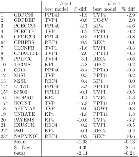
5.1 RMSE Results

To summarize the contents of Tables 13 and 14, we provide in Table 5 the list of the best

model for each series, together with the relative performance of the best break model with

respect to the best no-break model. It appears that according to the RMSE criterion, at

horizon one, the break models are the best in 83 percent of all series (26 for PPT, 22 for

KP1, and 35 for TVP1). At horizon four, the break models forecast better in 70 percent (30

for PPT1, 10 for KP1, and 30 for TVP1). REC is best for four series at horizon one and

five at horizon four, ROW is best only for one series at horizon four, and UC-SV as well.

These scores do not take account of the magnitude of the differences of the RMSE between

the different models (for this see below). Though there are many cases where the best model

differs between horizons one and four, a switch between a break model and a no-break one

happens in seven series on a total of twenty-three.

With the results in Tables 5–13-14, we can answer to our questions about the forecasting

performance of the different models.

Question 1: To answer, we compare the best break model RMSE value to the best no-break

best break (no-break) model has its RMSE three percent smaller (larger) than the RMSE of

the best no-break (break) model. Although for a high proportion of the series the differences

are negative, they are nevertheless small, by what we mean they are less than five percent

(often much less). Exceptions are, at horizon one, series 10 (-6 for KP1), 17 (-18 for TVP1),

and 20 (-11 for KP4). At horizon four, one difference is larger than 5 (series 10, +11 for

REC4). A test for the nullity of the mean of the differences is significant at the five percent

level for horizon one, but not for horizon four. In brief, there is some weak evidence in our

results that break models perform a little better than no-break models.

Table 5: Relative performance of best forecasting models on last thirty percent of sample

(Root mean squared error criterion)

h= 1 h= 4

best model % diff. best model % diff

1 GDPC96 PPT41 -1.9 TVP4 -2.9

2 GDPDEF TVP4 -0.6 UC-SV 2.0

3 PCECC96 PPT40 -2.7 KP4 -4.6

4 PCECTPI TVP1 -1.2 TVP1 -0.2

5 GPDIC96 PPT40 -0.3 PPT10 -0.8

6∗ _{OPHPBS REC4 0.2 REC4 0.1}

7 ULCNFB TVP1 -1.6 TVP1 -0.3

8 CPIAUCSL TVP4 2.0 PPT10 -0.3

9 PPIFCG TVP4 3.1 REC4 -0.6

10 TB3MS KP1 -5.8 REC4 0.2

11 GS10 PPT40 -0.4 PPT40 -0.3

12 M1SL TVP1 -0.3 PPT11 -0.2

13 M2SL REC4 0.4 KP1 0.0

14∗ _{UTL11 PPT40 -3.5 PPT40 -1.6}

15∗ _{SP500 PPT11 -0.1 TVP1 -0.5}

16 INDPRO KP4 -1.4 TVP4 -1.3

17∗ _{HOUST TVP1 -17.8 PPT11 -1.0}

18 AHEMAN TVP1 -0.6 ROW4 0.3

19 UNRATE KP4 -1.8 PPT41 1.8

20 PAYEMS KP4 -10.6 TVP4 -3.2

21 EXUSUK REC4 0.2 TVP1 -0.5

22∗ _{PMI KP4 -0.1 REC4 0.2}

23∗ _{NAPMNOI REC4 0.2 REC4 10.6}

Mean -1.93 -0.13

St. Dev. 4.39 2.75

t-stat -2.11 -0.24

Source: results in Tables 13-14. See Table 4 for definitions of mod-els. The ”%diff” are computed as [(smallest RMSE across the break models/smallest RMSE across the no-break models)-1]x100.

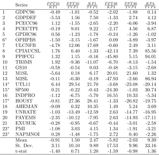
are shown in Table 6. For example, the value -0.49 of series 1 for a comparison of PPT10

and KP1 means that PPT10 is performing better than KP1 by almost half a percent. Means

and standard deviations are given at the bottom of each column. The results show that for

most series the differences are small, and there are a few cases where they are large. On

average, at horizon one, PPT performs slightly better than KP, and TVP better than the

other two models. At horizon four, PPT performs better on average than the other two

models, and TVP dominates KP. Nevertheless given the large standard deviations due to a

few large differences, no mean is significant even at the ten percent level.

Table 6: Performance comparison of break models on last thirty percent of sample

(Root mean squared error criterion)

Series P P T10

K P1

P P T10

T V P1

K P1

T V P1

P P T40

K P4

P P T40

T V P4

K P4

T V P4

1 GDPC96 -0.49 -1.01 -0.52 -2.02 -1.88 0.14

2 GDPDEF -5.53 1.56 7.50 -1.33 2.74 4.12

3 PCECC96 1.12 -1.55 -2.65 -2.20 -6.06 -3.94

4 PCECTPI -0.19 9.01 9.22 -2.17 4.56 6.87

5 GPDIC96 0.56 -1.23 -1.78 -0.24 -1.26 -1.02

6∗ _{OPHPBS -1.50 -3.15 -1.67 0.09 -3.89 -3.97}

7 ULCNFB -4.78 12.06 17.69 -0.60 2.49 3.11

8 CPIAUCSL 1.76 0.40 -1.33 -42.13 7.39 85.56

9 PPIFCG 1.32 1.15 -0.16 -45.80 5.15 94.01

10 TB3MS 1.92 -9.36 -11.07 -6.70 -8.13 -1.54

11 GS10 -0.58 -0.54 0.03 -0.48 -3.15 -2.68

12 M1SL -5.64 0.18 6.17 20.01 21.60 1.32

13 M2SL -0.11 -0.30 -0.19 -47.93 -2.66 86.94

14∗ _{UTL11 6.44 29.54 21.70 -3.68 -23.08 -20.14}

15∗ _{SP500 0.21 -0.22 -0.43 -24.30 -1.03 30.74}

16 INDPRO -1.12 -6.75 -5.70 16.55 10.33 -5.34

17∗ _{HOUST -0.81 27.36 28.41 -1.33 -20.82 -19.75}

18 AHEMAN -9.09 0.32 10.35 1.49 5.24 3.69

19 UNRATE -1.03 -13.49 -12.59 2.63 -14.77 -16.95

20 PAYEMS -2.35 -10.12 -7.95 2.63 -14.93 -17.11

21 EXUSUK -0.28 -0.95 -0.67 -0.44 -3.01 -2.58

22∗ _{PMI -1.08 3.03 4.15 1.34 -1.91 -3.21}

23∗ _{NAPMNOI 0.28 -1.48 -1.75 2.72 0.40 -2.26}

Mean -0.91 1.50 2.47 -5.82 -2.03 9.39

St. Dev. 3.11 10.10 9.89 17.53 9.96 33.16

t-stat -1.40 0.71 1.20 -1.59 -0.98 1.36

Source: results in Tables 13-14. See Table 4 for definitions of models. The values for column header A

B are computed as [(RMSE of model A/RMSE of

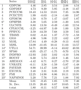
are reported in Table 7. These results indicate that the models with four lags perform a

little better than those with one lag, maybe not a surprise for quarterly data. However, the

differences are significant at the ten percent level on average only for PPT and REC.

Another question of interest is whether allowing for a possible single break (rather than no

break) in the forecast period makes a difference in the PPT approach. Pesaran, Pettenuzzo,

and Timmermann (2006) found on their example (a single series) that this decreases RMSE at

all horizons on their full sample and on several subsamples. We don’t find this to be significant

on average for our series with one lag (t-stat−0.05 at horizon 1 and 0.81 at horizon four), but with four lags there is some evidence in favor of allowing for a possible break: the performance

is improved on average by 0.49 percent at horizon 1 (t-stat 1.91) and by 2 percent at horizon

four (t-stat 1.75).

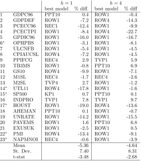
5.2 APL Results

We summarize the contents of Tables 15 and 16 in Table 8 where we list the best model for

each series, together with the relative performance of the best break model with respect to

the best no-break model. It appears that according to the APL criterion, at horizon one,

the break models are the best in 22 percent of all series (9 for PPT, 4 for KP1, and 9 for

TVP1). At horizon four, the break models forecast better also in 22 percent (13 for PPT1, 0

for KP1, and 9 for TVP1). ROW is the best at horizon one for fourteen series (61 percent)

and seventeen (74 percent) at horizon four. REC is the best for four series at horizon one

and one at horizon four, and UC-SV is dominated by all other models. These scores do not

take account of the magnitude of the differences of the APL between the different models

but suggest that ROW is by far dominating the other models (for this see question 1 below).

Though there are many cases where the best model differs between horizons one and four,

a switch between a break model and a no-break model happens in six series on a total of

twenty-three.

With the results in Tables 8–15-16, we can answer to our questions about the forecasting

performance of the different models.

Question 1: To answer, we compare the best break model APL value to the best no-break

model value, see columns ”% diff.” in Table 8. For example, a value of +4 (-4) means that

no-Table 7: Performance comparison of lag orders on last thirty percent of sample

(Root mean squared error criterion)

Series P P T10

P P T40

K P1

K P4

T V P1

T V P4

ROW1

ROW4

REC1

REC4

1 GDPC96 4.46 2.85 3.54 2.88 4.54

2 GDPDEF 4.73 9.39 5.95 -3.48 11.67

3 PCECC96 18.43 14.53 13.01 7.35 14.96

4 PCECTPI 1.99 -0.03 -2.18 -1.60 2.87

5 GPDIC96 1.50 0.70 1.47 -3.07 1.87

6∗ _{OPHPBS 3.38 5.05 2.59 -1.20 3.85}

7 ULCNFB 8.80 13.58 -0.49 -1.60 12.54

8 CPIAUCSL -3.25 -44.97 3.49 1.00 3.29

9 PPIFCG 3.59 -44.59 7.68 3.59 7.65

10 TB3MS 0.02 -8.44 1.37 -7.72 -1.58

11 GS10 4.96 5.06 2.22 4.62 4.97

12 M1SL -17.84 4.49 -0.28 -9.13 -0.82

13 M2SL 13.09 -41.05 10.41 11.03 13.57

14∗ _{UTL11 54.71 39.99 -8.14 43.62 40.93}

15∗ _{SP500 -0.95 -25.17 -1.75 -9.70 -2.74}

16 INDPRO -12.93 2.63 3.02 -4.10 5.94

17∗ _{HOUST 6.30 5.74 -33.9 1.46 5.61}

18 AHEMAN -4.42 6.71 0.27 -2.70 17.20

19 UNRATE -0.11 3.58 -1.59 -5.87 -1.48

20 PAYEMS 8.90 14.47 3.08 4.27 2.60

21 EXUSUK 2.48 2.31 0.35 2.19 2.25

22∗ _{PMI 12.25 14.98 6.86 10.11 13.91}

23∗ _{NAPMNOI 5.20 7.76 7.21 1.88 7.92}

Mean 5.01 -0.45 1.05 1.91 7.46

St. Dev. 13.35 20.40 8.87 10.65 9.25

t-stat 1.80 -0.11 0.57 0.86 3.87

Source: results in Tables 13-14. See Table 4 for definitions of mod-els. The values for column header A

B are computed as [(RMSE of

Table 8: Relative performance of best forecasting models on last thirty percent of sample

(Average predictive likelihood criterion)

h= 1 h= 4

best model % diff. best model % diff

1 GDPC96 PPT10 0.4 ROW1 -0.4

2 GDPDEF ROW1 -7.2 ROW4 -14.3

3 PCECC96 REC1 -12.4 ROW1 -9.9

4 PCECTPI ROW1 -8.4 ROW4 -22.7

5 GPDIC96 ROW1 -16.0 ROW1 -16.7

6∗ _{OPHPBS ROW1 -3.1 ROW1 -8.1}

7 ULCNFB ROW1 -5.4 ROW1 -4.5

8 CPIAUCSL ROW4 -7.2 ROW1 -4.5

9 PPIFCG REC4 2.9 TVP1 5.9

10 TB3MS ROW1 -0.8 PPT10 6.9

11 GS10 ROW4 -9.9 ROW1 -7.1

12 M1SL REC4 -1.7 REC4 -2.6

13 M2SL TVP4 2.7 ROW1 -1.2

14∗ _{UTL11 ROW4 -17.8 ROW1 -1.6}

15∗ _{SP500 KP1 0.7 PPT10 0.1}

16 INDPRO TVP1 7.8 TVP1 9.7

17∗ _{HOUST ROW1 -19.0 ROW4 -13.6}

18 AHEMAN PPT10 0.1 ROW1 -0.7

19 UNRATE ROW1 -14.2 ROW1 -15.5

20 PAYEMS ROW1 1.6 PPT10 6.8

21 EXUSUK ROW1 -2.5 ROW1 0.5

22∗ _{PMI ROW4 -13.4 ROW1 -9.1}

23∗ _{NAPMNOI REC4 -0.6 ROW1 -3.9}

Mean -5.36 -4.64

St. Dev. 7.40 8.31

t-stat -3.48 -2.68

Source: results in Tables 15-16. See Table 4 for definitions of mod-els. The ”%diff” are computed as [(largest APL across the break models/largest APL across the no-break models)-1]x100.

break (break) model. At horizon one, the differences are larger than five percent in absolute

value for twelve series, and only for one (series 16) the difference is positive. At horizon four,

nine differences are smaller than minus five percent and four are larger than five percent. A

test for the nullity of the mean of the differences is significant at the one percent level for both

horizons. In brief, there is strong evidence in our results that the no-break models (especially

ROW) perform much better than break models, though there are a few exceptions (series 16

at both horizons, series 9, 10 and 20 at horizon four).

Question 2: The relative differences (in percent) between the APL of the different models

KP1 means that PPT10 is performing better than KP1 by a little more than 8 percent. The

differences vary a lot, and there are a few cases where they are very large. On average, at

both horizons, PPT performs slightly better than KP but not significantly even at the ten

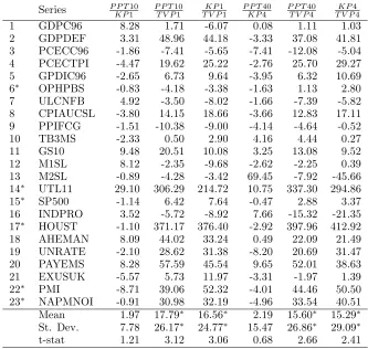
percent level, and TVP is significantly dominated by the other two models.

Table 9: Performance comparison of break models on last thirty percent of sample

(Average predictive likelihood criterion)

Series P P T10

K P1

P P T10

T V P1

K P1

T V P1

P P T40

K P4

P P T40

T V P4

K P4

T V P4

1 GDPC96 8.28 1.71 -6.07 0.08 1.11 1.03

2 GDPDEF 3.31 48.96 44.18 -3.33 37.08 41.81

3 PCECC96 -1.86 -7.41 -5.65 -7.41 -12.08 -5.04

4 PCECTPI -4.47 19.62 25.22 -2.76 25.70 29.27

5 GPDIC96 -2.65 6.73 9.64 -3.95 6.32 10.69

6∗ _{OPHPBS -0.83 -4.18 -3.38 -1.63 1.13 2.80}

7 ULCNFB 4.92 -3.50 -8.02 -1.66 -7.39 -5.82

8 CPIAUCSL -3.80 14.15 18.66 -3.66 12.83 17.11

9 PPIFCG -1.51 -10.38 -9.00 -4.14 -4.64 -0.52

10 TB3MS -2.33 0.50 2.90 4.16 4.44 0.27

11 GS10 9.48 20.51 10.08 3.25 13.08 9.52

12 M1SL 8.12 -2.35 -9.68 -2.62 -2.25 0.39

13 M2SL -0.89 -4.28 -3.42 69.45 -7.92 -45.66

14∗ _{UTL11 29.10 306.29 214.72 10.75 337.30 294.86}

15∗ _{SP500 -1.14 6.42 7.64 -0.47 2.88 3.37}

16 INDPRO 3.52 -5.72 -8.92 7.66 -15.32 -21.35

17∗ _{HOUST -1.10 371.17 376.40 -2.92 397.96 412.92}

18 AHEMAN 8.09 44.02 33.24 0.49 22.09 21.49

19 UNRATE -2.10 28.62 31.38 -8.20 20.69 31.47

20 PAYEMS 8.28 57.59 45.54 9.65 52.01 38.63

21 EXUSUK -5.57 5.73 11.97 -3.31 -1.97 1.39

22∗ _{PMI -8.71 39.06 52.32 -4.01 44.46 50.50}

23∗ _{NAPMNOI -0.91 30.98 32.19 -4.96 33.54 40.51}

Mean 1.97 17.79∗ _16.56∗ _{2.19 15.60}∗ _15.29∗

St. Dev. 7.78 26.17∗ _24.77∗ _{15.47 26.86}∗ _29.09∗

t-stat 1.21 3.12 3.06 0.68 2.66 2.41

Source: results in Tables 15-16. See Table 4 for definitions of models. The values for column header A

B are computed as [(APL of model A/APL of model

B)-1]x100. Means and standard deviations with a∗superscript are computed

excluding the values for series 14 and 17.

Question 3: The relative differences (in percent) between the RMSE of the different models

are reported in Table 7. On average models with four lags do not perform better than models

Allowing for one break deteriorates the performance on average: with one lag by 0.68 percent

at horizon one (t-stat −5.29) and 5.42 percent at horizon four (t-stat −6.65); with four lags by 0.93 percent at horizon one (t-stat −6.05) and 8.40 percent at horizon four (t-stat 14.4). This is is explained by the increase of the predictive variances when one break is allowed,

while the predictive means do not change much as witnessed by the RMSE results.

Table 10: Performance comparison of lag orders on last thirty percent of sample

(Average predictive likelihood criterion)

Series P P T10

P P T40

K P1

K P4

T V P1

T V P4

ROW1

ROW4

REC1

REC4

1 GDPC96 4.36 -3.54 3.75 5.41 -1.57

2 GDPDEF 7.34 0.43 -1.22 0.80 -4.74

3 PCECC96 -4.93 -10.31 -9.73 -7.72 -4.16

4 PCECTPI -5.97 -4.29 -1.19 4.55 -6.49

5 GPDIC96 3.27 1.89 2.87 4.61 -1.80

6∗ _{OPHPBS -2.70 -3.48 2.69 2.74 -3.98}

7 ULCNFB 2.43 -4.00 -1.70 4.75 -7.28

8 CPIAUCSL -5.73 -5.58 -6.82 -3.42 -8.66

9 PPIFCG -2.48 -5.09 3.77 -2.42 -4.42

10 TB3MS 1.73 8.49 5.71 5.43 -3.27

11 GS10 1.03 -4.73 -5.21 -2.64 -2.10

12 M1SL 6.39 -4.17 6.50 6.41 -1.69

13 M2SL -7.51 58.12 -11.03 -5.85 -8.81

14∗ _{UTL11 -7.43 -20.59 -0.36 -19.11 -21.82}

15∗ _{SP500 3.99 4.69 0.54 3.33 2.86}

16 INDPRO 11.49 15.95 0.14 7.18 -7.98

17∗ _{HOUST -1.42 -3.23 4.18 1.49 -2.75}

18 AHEMAN 12.61 4.69 -4.54 1.50 -16.72

19 UNRATE 6.24 -0.39 -0.32 6.15 1.41

20 PAYEMS 9.17 10.55 5.30 3.91 -3.60

21 EXUSUK 7.73 10.31 -0.11 6.83 0.57

22∗ _{PMI -7.62 -2.87 -4.03 -6.47 -10.15}

23∗ _{NAPMNOI -1.09 -5.13 0.84 3.85 -5.43}

Mean 1.34 1.64 -0.43 0.92 -5.33

St. Dev. 6.26 14.52 4.74 6.25 5.54

t-stat 1.03 0.54 -0.44 0.71 -4.61

Source: results in Tables 15-16. See Table 4 for definitions of mod-els. The values for column header A

B are computed as [(APL of

model A/APL of model B)-1]x100.

5.3 Discussion of Previous Results

For the APL criterion and the last thirty percent of the sample that serves as forecast period,

break models. For the RMSE criterion, we find some weak evidence in favor of break models.

Why this difference?

The APL criterion takes into account the whole shape of the predictive density. This

is not normal despite the assumption of normality (conditional on the parameters), because

it is integrated with respect to a posterior distribution that is not symmetric. However our

predictive densities are very moderately skewed since we forecast at short horizons. Therefore,

we can summarize the shape of our predictive by their standard deviation. The RMSE results

indicate that in terms of the location of the point forecasts in the support of the predictive

densities, the two kinds of models (break/no-break) are roughly equivalent on average (of

course, individual exceptions occur). Thus logically the differences in the APL results must

be (at least partly) due to differences in the standard deviation of the predictive densities. In

the results, we find some weak evidence that supports our explanation.

Our rationale uses estimation results reported in Table 3 for the PPT- and KP-AR(1)

models and also for the no-break AR(1) models estimated with an expanding window (AR(1)

full sample header, named REC hereafter) and a rolling window of forty observations (AR(1)

last forty data, named ROW1 hereafter). For the latter, in the last three columns of the table,

we report two sets of point estimates: on the first row the estimates are computed with the

last forty observations of the full sample, on the second row (in italics), they are computed

with the last forty observations of the sample that ends just before the forecast period begins

(1995). We call the latter the pre-forecast sample. For example, for series 1, the posterior

expectation of the error variance is equal to 0.36 for the last forty observations of the full

sample, 0.26 for the pre-forecast sample, and 0.69 for the full sample.

If we compare the pre-forecast ROW1 variance estimates with those of the regime

gener-ating the PPT and KP forecasts, we find that for most series the ROW1 estimate is smaller

than the PPT, KP, or even REC estimates.6

This is nothing else but the effect of the great

moderation. Since the variance of the error determines to a large extent the predictive

vari-ance, we expect that that for the series witnessing this effect, the predictive densities are more

concentrated when based on estimates using essentially data in that period than using data

starts in the mid-eighties and our forecast period starts about ten years later). Thus for an

observation that is not far from the mean, the predictive density of ROW1 should be larger

than the predictive of PPT, if the predictive densities have similar means. For an observation

far in the tails, the reverse is true. We indeed observe this on many graphs of predictive

densities. Hence if the observations of the forecast sample are not outliers in the predictive,

and the predictive of both models have approximately the same mean at every date, the APL

of ROW1 should be larger than the APL of PPT.7

To be concrete on this, let us compare the σ2

estimate that is effective at the beginning

of the forecast period from PPT-AR(1) with the σ2 _{estimate from the AR(1) model on the}

pre-forecast period. The error variance estimates of AR(1) models are smaller on average

by 17.45 percent (t-stat −2.42). A comparison of the APL values reveals that they increase on average by 8.91 percent (t-stat. 4.25) at horizon one, and by 8.42 percent (t-stat 3.26)

at horizon four. The correlation coefficients between the series of percentage changes of the

variances and of the APL are, as expected, negative:−0.21 (t-stat −0.98) for horizon one, and −0.29 (t-stat−1.41) for horizon four. These negative correlations support our previous explanation of why ROW1 performs better than PPT in terms of APL, though they are

not much significant statistically (the p-values of the t-statistics are 0.33 and 0.17). Similar

computations with KP-AR(1) instead of PPT10-AR(1) give similar results, with correlations

of −0.21 (t-stat−0.72) at horizon one and−0.14 (t-stat−2.01) at horizon four.

6

Sensitivity Analyses

We perform two sensitivity checks. The first is with respect to the forecast period: we focus

on the last three years of data, starting in 2007, quarter three, which corresponds more or

less to the beginning of the great recession, until the end of the sample. The second check

7_{A similar argument applies if we compare the APL of PPT10 and PPT11 (and also PPT40 with PPT41).}

concerns the influence of the prior used in the break models.

6.1 Forecast performance since the middle of 2007

These results were obtained with the same prior as in the previous section. We focus on

ques-tion 1 since for the other quesques-tions the previous answers are unchanged, with the excepques-tion

that for question 2, using the RMSE criterion, PPT performs significantly better on average

than KP at both horizons.

For the RMSE criterion, break models perform better than no-break models in about

eighty percent of series at both horizons and on average (see the negative means in Table 11).

These differences are significant on average at the five percent level, as the t-statistics in the

table reveal. This is stronger than in the results for the last thirty percent of the sample (see

subsection 5.1).

For the APL criterion, we find that break models perform better than no-break models

in about fifty percent of series at horizon 1, and the (slightly negative) mean difference is

not significant. At horizon four, break models dominate in about eighty percent of series and

the mean difference (of almost +12 percent) is significant at the one percent level. These

conclusions are different from what we found for the last thirty percent of the sample, where

the no-break models, especially ROW, were clearly the winners (see subsection 5.2).

We can explain the improved performance of the break models with respect to ROW

for the last twelve observations by the same argument as in subsection 5.3, but reversed.

Estimated error variances (by ROW) increase at the end of the sample8

due to the impact of

the financial crisis, while break models do not capture this as much (few series have a break

around mid-2007).

6.2 Impact of the prior for break models

In Bayesian inference, it is good practice to assess the sensitivity of the results with respect

to the informative content of the prior. Thus we have computed again all the results with

different sets of prior hyperparameters, one implying a more informative prior (PRIOR M),

Table 11: Performance comparison on last twelve observations

RMSE APL

% diff. h= 1 h= 4 h= 1 h= 4 Mean -15.8 -8.51 -0.12 11.96 t-stat -2.40 -2.19 -0.07 3.58

Source: results available on request. Mean is the mean of percentage differences of the series.

of PRIOR I are given in Appendix A for the PPT model and in Appendix B for the KP

model.

All our priors (M, I, L) imply that the unconditional prior expectations are equal to

zero for the regression coefficients of the AR(1) or AR(4) equations in each regime since

E(βj) =E[E(βj|β0)] =E(β0) and the latter is set to zero. They imply non-existing second

moments for the regression coefficients because V ar(βj) =V ar[E(βj|β0)] +E[V ar(βj|β0)] =

V ar(β0) +E(B0) andE(B0) is not finite due to setting the degrees of freedom of the Wishart

prior to m+ 1, withm= 2 for AR(1) and 5 for AR(4). However V ar(β0) is set tocIm with

c = 1 in PRIOR I and by changing the value of c, we can change the tightness of the prior

on the regression coefficients.

In PRIOR L, we setc= 100, implying standard deviations equal to 10 forβ0, that is ten

times larger than the corresponding value in PRIOR I (which has c = 1). We are also less

informative on error variances of AR equations by setting ρ= 0.01 and d= 0.01 (instead of

0.1 for both in PRIOR I) in the PPT model. In the KP model, we setV_ω = 100 (instead of

1) andκ1=κ2 = 0.01 (instead of 0.5).

In PRIOR M, we setc= 0.01Im, implying a more precise prior (with standard deviations

of 0.1) than in PRIOR I. For the other parameters of the prior, the values are the same as in

PRIOR I.

Computed by simulation, the highest prior density interval of ninety percent level for

each regression coefficient is equal to (−17,+17) for PRIOR L, (−3.9,+3.9) for PRIOR I, and (−2.6,+2.6) for PRIOR M. Notice that if c is set to a smaller value than 0.01, the last interval does not shrink due to the E(B0) term that is not finite. Compared to the