Selection of Heteroscedastic Models: A Time Series Forecasting Approach

(1)

ISSN Online: 2152-7393 ISSN Print: 2152-7385

DOI: 10.4236/am.2019.105024 May 23, 2019 333 Applied Mathematics

Selection of Heteroscedastic Models: A Time

Series Forecasting Approach

Imoh Udo Moffat

1

, Emmanuel Alphonsus Akpan

2

1_{Department of Mathematics and Statistics, University of Uyo, Uyo, Nigeria}

2_{Department of Mathematical Science, Abubakar Tafawa Balewa University, Bauchi, Nigeria}

Abstract

To overcome the weaknesses of in-sample model selection, this study adopted out-of-sample model selection approach for selecting models with improved forecasting accuracies and performances. Daily closing share prices were ob-tained from Diamond Bank and Fidelity Bank as listed in the Nigerian Stock Exchange spanning from January 3, 2006 to December 30, 2016. Thus, a total of 2713 observations were explored and were divided into two portions. The first which ranged from January 3, 2006 to November 24, 2016, comprising 2690 observations, was used for model formulation. The second portion which ranged from November 25, 2016 to December 30, 2016, consisting of 23 observations, was used for out-of-sample forecasting performance evalua-tion. Combined linear (ARIMA) and Nonlinear (GARCH-type) models were applied on the returns series with respect to normal and student-t distribu-tions. The findings revealed that ARIMA (2,1,1)-EGARCH (1,1)-norm and ARIMA (1,1,0)-EGARCH (1,1)-norm models selected based on minimum predictive errors throughout-of-sample approach outperformed ARIMA (2,1,1)-GARCH (2,0)-std and ARIMA (1,1,0)-EGARCH (1,1)-std model cho-sen through in-sample approach. Therefore, it could be deduced that out-of-sample model selection approach was suitable for selecting models with improved forecasting accuracies and performances.

Keywords

ARIMA Model, GARCH-Type Model, Heteroscedasticity, Model Selection, Time Series Forecasting, Volatility

1. Introduction

Model selection is the act of choosing a model from a class of candidate models as a quest for a true model or best forecasting model or both (see also, [1], [2],

How to cite this paper: Moffat, I.U. and Akpan, E.A. (2019) Selection of Heteros-cedastic Models: A Time Series Forecast-ing Approach. Applied Mathematics, 10, 333-348.

https://doi.org/10.4236/am.2019.105024

Received: April 15, 2019 Accepted: May 20, 2019 Published: May 23, 2019

http://creativecommons.org/licenses/by/4.0/

(2)

DOI: 10.4236/am.2019.105024 334 Applied Mathematics

[3]). There are often several competing models that can be used for forecasting a particular time series. Consequently, selecting an appropriate forecasting model is considerably practical importance [4] [5]. Selecting the model that provides the best fit to historical data generally does not result in a forecasting method that produces the best forecasts of new data. Concentrating too much on the model that produces the best historical fit often leads to overfitting, or including too many parameters or terms. The best approach is to select the model that re-sults in the smallest standard deviation or mean squared error of the one-step-ahead forecast errors when the model is applied to data set that was not used in fitting process [4]. There are two approaches to model selection in time series; the in-sample model selection and the out-of-sample model selection. The in-sample model selection is targeted at selecting a model for inference, which according to [1] is intended to identify the best model for the data and to pro-vide a reliable characterization of the sources of uncertainty for scientific insight and interpretation. The sample model selection criteria include Akaike in-formation criterion, AIC [6], Schwarz information criterion, SIC [7], and Han-nan and Quinn information criteria, HQIC [8]. As captured in [9], AIC consi-dered a discrepancy between the true model and a candidate, BIC approximated the posterior model probabilities in a Bayesian framework, and Hannan and Quinn proposed a related criterion which has a smaller penalty compared to BIC that yet permitted strong consistency property (for more details on information criteria, see [10] [11] [12] [13] [14]). However, the major drawbacks of in-sample model selection criteria are that, they are unstable and minimizing these criteria over a class of candidate models leads to a model selection proce-dure that is conservative or over-consistent in parameter settings [2] [9], and the inability to inform directly about the quality of the model [3]. On the other hand, out-of-sample model selection procedure is applied to achieve the best predictive performance, essentially at describing the characterization of future observations without necessarily considering the choice of true model, rather, the attention is shifted to choose a model with the smallest predictive errors [1] [2] [15] [16]. The out-of-sample forecast is accomplished when the data used for constructing the model are different from that used in forecasting evaluation. That is, the data is divided into two portions. The first portion is for model con-struction and the second is used for evaluating the forecasting performance with possibility of forecasting new future observations which can be checked against what is observed ([11] [16] [17]). Yet the choice of in-sample and out-of-sample model selection criteria is not without contention and such contention is well handled in [1] [15] [18] [19] [20].

(3)

fitted heteroscedastic models by adopting out-of-sample forecasting approach in selecting heteroscedastic models that would best describe the accuracy and pre-cision of future observations.

This work is further organized as follows: materials and methods are treated in Section 2, results and discussion covered in Section 3 and Section 4 takes care of conclusion.

2. Materials and Methods

2.1. Return

The return series Rt can be obtained given that Pt is the price of a unit share at time t, and Pt−1 is the share price at time t−1.

(

)

1

ln 1 ln ln ln

t t t t t

R = ∇ P = −B P = P− P− (1)

The Rt in Equation (1) is regarded as a transformed series of the share price, t

P meant to attain stationarity, that is, both mean and variance of the series are stable [29]. The letter B is the backshift operator.

2.2. Information Criteria

There are several information criteria available to determine the order, p, of an AR process and the order, q, of MA(q) process, all of them are likelihood based. The well-known Akaike information criterion (AIC), [6] is defined as

(

)

(

)

2 2

AIC ln likelihood x number of parameters ,

T T

−

= + ₍₂₎

where the likelihood function is evaluated at the maximum likelihood estimates and T the sample size. For a Gaussian AR(p) model, AIC reduces to

( )

_ˆ2 2

AIC P =ln σP + _TP (3)

where _ˆ2

P

σ is the maximum likelihood estimate of _ˆ2

a

σ , which is the variance of

t

a , and T is the sample size. The first term of the AIC in Equation (6) measures the goodness-of-fit of the AR(p) model to the data whereas the second term is called the penalty function of the criterion because it penalizes a chosen model by the number of parameters used. Different penalty functions result in different information criteria.

The next commonly used criterion function is the Schwarz information crite-rion (SIC), [7]. For a Gaussian AR(p) model, the criterion is

( )

_ˆ2 ln

( )

SIC ln P

P T P

T

σ  

= +  

  (4)

Another commonly used criterion function is the Hannan Quinn information criterion (HQIC), [8]. For a Gaussian AR(p) model, the criterion is

( )

_ˆ2 ln ln

{

( )

}

HQIC ln P

T P

T

σ

= + ₍₅₎

(4)

for HQIC. These penalty functions help to ensure selection of parsimonious models and to avoid choosing models with too many parameters.

The AIC criterion asymptotically overestimates the order with positive proba-bility, whereas the BIC and HQIC criteria estimate the order consistently under fairly general conditions ([11] [17]). Moreover, an in-sample model selection criterion is consistent if it chooses a true model when the true model is among those considered with probability approaching unity as the sample size becomes large, and if the true model is not among those considered, it selects the best ap-proximation with probability approaching unity as sample size becomes larger [3]. The AIC is always considered inconsistent in that it does not penalize the inclusion of additional parameters. As such, relying on these criterion leads to overfitting. Meanwhile, the SIC and HQIC criteria are consistent in that it takes into account large size adjustment penalty. In contrast, consistency is not suffi-ciently informative. It turns out that the true model and any reasonable ap-proximation to it are very complex. An asymptotically efficient model selection criterion chooses a sequence of models as the sample size get larger for which the one-step-ahead forecast error variances approach the one-step-ahead fore-cast error variance for the true model at least as fast as any other criterion [3]. The AIC is asymptotically efficient while SIC and HQIC are not. However, one major drawback of in-sample criteria is their inability to evaluate a candidate model’s potential predictive performance.

2.3. Model Evaluation Criteria

It is tempting to evaluate performance on the basis of the fit of the forecasting or time series model to historical data [3]. The best way to evaluate a candidate model’s predictive performance is to apply the out-of-sample forecast technique. This will provide a direct estimate of the one-step-ahead forecast error variance that guarantees an efficient model selection criterion. The methods of forecast evaluation based on forecast error include Mean Squared Error (MSE), Root Mean Squared Error (RMSE) and Mean Absolute Error (MAE). These criteria measure forecast accuracy. The forecast bias is measured by Mean Error (ME).

The measures are computed as follows:

2 1 1

MSE=_n

∑

ni=ei (6)

2 1 1

RMSE= _n

∑

in=ei (7)

1 1

MAE= _n

∑

n_i= ei (8)

( )

1 1

ME n _i

i e

n =

=

∑

₍₉₎

(5)

2.4. Autoregressive Integrated Moving Average (ARIMA) Model

[10] considered the extension of ARMA model to deal with homogenous

non-stationary time series in which Xt, itself is non-stationary but its dth dif-ference is a stationary ARMA model. Denoting the dth_{difference of}

t

X by

( )

d

( )

,

t t

B B X B

ϕ =φ ∇ =θ ε ₍₁₀₎

where ϕ

( )

B _{is the nonstationary autoregressive operator such that}_d_{of the}

roots of ϕ

( )

B =0 are unity and the remainder lie outside the unit circle.

( )

B

φ _{is a stationary autoregressive operator.}

2.5. Heteroscedastic Models

Autoregressive Conditional Heteroscedastic (ARCH) Model: The first model that provides a systematic framework for modeling heteroscedasticity is the ARCH model of [35]. Specifically, an ARCH (q) model assumes that,

, ,

t t t t t t

R =µ +a a =σ e

2 2 2

1 1

t at q t qa

σ = +ω α − + + α − , (11)

where

[ ]

et is a sequence of independent and identically distributed (i.i.d.) ran-dom variables with mean zero, that is E

( )

et =0 and variance 1, that is

( )

2

E et =1,

ω

>0, and α1, ,α ≥q 0 [36]. The coefficients αi, for i>0, must satisfy some regularity conditions to ensure that the unconditional va-riance of at is finite.

Generalized Autoregressive Conditional Heteroscedastic (GARCH) Mod-el: Although the ARCH model is simple, it often requires many parameters to adequately describe the volatility process of a share price return. Some alterna-tive models must be sought. [37] proposed a useful extension known as the ge-neralized ARCH (GARCH) model. For a return series, Rt, let at =Rt−µt be the innovation at time t. Then, at follows a GARCH(q, p) model if

t t t

a =σe_,

2 2 2

1 1 ,

q q

t i t i j t j

i a j

σ ω α ₋ β σ₋

= =

= +

∑

+

∑

₍₁₂₎

where again et is a sequence of i.i.d. random variance with mean, 0, and

va-riance, 1, ω>0,αi ≥0,βj ≥0, and

(

)

( )

max ,

1 1

p q

i i

i

α β =

+ <

∑

(see [38]).

Here, it is understood that α =i 0, for i p> , and β =i 0, for i q> . The latter constraint on α βi+ i implies that the unconditional variance of at is fi-nite, whereas its conditional variance 2

t

σ , evolves over time.

Exponential Generalized Autoregressive Conditional Heteroscedastic (EGARCH) Model: The EGARCH model represents a major shift from ARCH and GARCH models [39]. Rather than modeling the variance directly, EGARCH models the natural logarithm of the variance, and so no parameter restrictions are required to ensure that the conditional variance is positive. The EGARCH(q,

(6)

, ,

t t t t t t

R =µ +a a =σ e

2 2

1 ₂ 1 ₂ 1

ln q t i r t k p ln ,

t i i k k j j t j

t i t k

a a

σ ω α γ β σ

σ σ − − − = = = − −     = + + +    

∑

(13)

where again, et is a sequence of i.i.d. random variance with mean, 0, and va-riance, 1, and γk is the asymmetric coefficient.

Glosten, Jagannathan and Runkle (GJR-GARCH) Model: The GJR-GARCH (q, p) model proposed by [40] is a variant, represented by

,

t t t

a =σ e

2 2 2 2

1 1 1 ,

q p p

t i i t ia i i t i t iI a j j t j

σ

= +

ω

∑

₌

α

₋ +

∑

₌

γ

₋ ₋ +

∑

₌

β σ

₋ ₍₁₄₎

where It−1 is an indicator for negative at i− , that is,

1

0 if 0, 1 if 0,

t i t t i a I a − − − <  =  _≥ 

and α γi, i and βj are nonnegative parameters satisfying conditions similar to those of GARCH models. Also the introduction of indicator parameter of leve-rage effect, It−1 in the model accommodates the leverage effect, since it is

sup-posed that the effect of 2

t i

a− on the conditional variance σt2 is different accor-dingly to the sign of at i− .

2.6. Parametric Bootstrap

The parametric bootstrap is used in computing nonlinear forecasts given the fact that the model used in forecasting has been rigorously checked and is judged to be adequate for the series under study [39]. Let T be the forecast origin and k be the forecast horizon (k > 0). That is, we are at time index T and interested in fo-recasting RT k+ . The parametric bootstrap considered compute realizations

1, ,

T T k

R +  R+ sequentially by drawing a new innovation from the specific inno-vational distribution of the model, and computing RT i+ using the model, data, and previous forecasts RT+1, , RT i+ −1. This results in a realization for RT k+ . The procedure is repeated M times to obtain M realizations of RT k+ denoted by

( )

{ }

_j M₁

T k j

R + ₌ . The point forecast of RT k+ is then the sample average of RT k( )+j .

Consequently, Forecasts of the ARCH model are obtained recursively. Let T

be the starting date for forecasting, that is forecast origin. Let FT be the infor-mation set available at time T. Then, the 1-step ahead forecast for conditional variance, 2

1

T σ ₊ _is

( )

2 2 2

1 1

ˆ ˆ ˆ ˆ ˆ

1 ,

T aT p Ta p

σ = +ω α + + α + − (15)

where aˆ_T is the estimated residual. For the 2-step ahead forecast 2 2

T σ ₊ _{, we} need a forecast of 2

1

T

a + . It is given by σT2

( )

1 . We therefore obtain

( )

2 2 2 2

1 2 2

ˆ ˆ ˆ ˆ ˆ ˆ

2 1 .

T T aT p Ta p

σ = +ω α σ +α + +_ α _{+ −} ₍₁₆₎

The k-step ahead forecast for 2

T k σ ₊ is

( )

(

)

(

)

2 2 2

1

ˆ ˆ 1 ˆ ,

T k T k p T k p

(7)

with 2

(

)

_ˆ2

T k i aT k i

σ − = + − if k i− ≤0.

Forecasts of the GARCH model are obtained recursively in a similar way as that of the ARCH model. Then, the 1-step ahead forecast for 2

1

T σ ₊ is

( )

2 2 2

1 ˆ1

ˆ ˆ ˆ ˆ

1

T aT T

σ = +ω α +β σ _{, (18)}

since 2 2 2

T T T

a =σ e _{, the GARCH (1,1) model can be rewritten as}

(

)

(

)

2 2 2 2 2 2

1 1 1 1 1 1 1 1 1 1 1

T aT T T T eT

σ

= +

ω α

₋ +

β σ

₋ = +

ω α β σ

+ ₋ +

α σ

₋ ₋ − _,

so that, at time T+2_{, we have}

(

)

(

)

2 2 2 2

2 1 1 1 1 1 1 1

T T T eT

σ

₊ = +

ω α β σ

+ ₊ +

α σ

₊ ₊ − _,

with

(

2

)

1 1 0

T T

E e_ + − F _= , we deduce the following 2-step ahead forecast for

2 2

T

σ ₊ _:

( )

(

)

( )

2 2

1 ˆ1 ˆ ˆ

2 1

T T

σ

= +

ω α β σ

+ _.

Generally speaking, the k-step ahead forecast for 2

T k σ ₊ _is

( )

(

)

(

)

2 2

1 ˆ1

ˆ ˆ 1 , 1.

T k T k k

σ

= +

ω α β σ

+ − > ₍₁₉₎

One of the beauties of GARCH is that volatility forecasts for any horizon can be constructed from the estimated model. The estimated GARCH model is used to get forecasts of instantaneous forward volatilities, that is, the forecast for

2

T k

σ ₊ made at time T and for every k step ahead.

For EGARCH model, assuming that the model parameters are known and the observations are standard Gaussian, for EGARCH (1,1) model, we have

(

)

( )

2 2

1 1 1 1

lnσT = −1 α ω α+ lnσT− +g T− ,

( )

T 1 T 1

(

T 1 2 π

)

g  ₋ =

θ

 ₋ +

γ

 ₋ − . (20)

Taking exponentials, the model becomes

(

)

( )

1 2 2

1exp 1 1 exp 1 ,

T Tα g T

σ

=

σ

₋ _ −

α ω

_ _ ₋ _

( )

T 1 T 1

(

T 1 2 π

)

g  ₋ =

θ

 ₋ +

γ

₋ − . (21)

For the 1-step ahead forecast, 2 1

T

σ + we have

( )

2 1

(

)

( )

2

1

1 exp 1 exp

T Tα g T

σ

=

σ

_ −

α ω

_ _ _ __{. (22)}

The 2-step-ahead forecast of 2 2

T

σ + is given by

( )

2 1

( )

(

)

{

( )

}

2

1 ˆ

2 1 exp 1 exp

T Tα ET g T

σ

=

σ

_ −

α ω

_ _  _ ,

where ET denotes a conditional expectation taken at the time origin T with

( )

{

}

(

)

( )2₂

₍

₎

( )2 ₂

₍

₎

exp T exp 2 π e e

E _g _ ₌ ₋

_γ

 θ γ+ _Φ

_{θ γ}

₊ ₊ θ γ− _Φ

_{γ θ}

₋ 

   _ _,

where Φ

( )

x is the cumulative density function of the standard normal distri-bution (see [39] for more details). Hence,

( )

(

)

(

)

(

)

(

)

(

)

{

}

1 2 2 1 2 2

ˆ 2 ˆ 1 exp 1 2π

exp 2 exp 2

T Tα

σ σ α ω γ

θ γ θ γ θ γ γ θ

 

= _ − − _

   

(8)

Generally, the k-step-ahead forecast can be obtained as

( )

(

)

(

)

(

)

(

)

(

)

(

)

{

}

1 2 2

1

2 2

ˆ ˆ 1 exp 1 2π

exp 2 exp 2

T k Tα k

σ σ α ω γ

θ γ θ γ θ γ γ θ

 

= − _ − − _

   

× _ + _Φ + + _ − _Φ − (23)

(See also, [34], [38]).

3. Results and Discussion

3.1. Plot Analysis

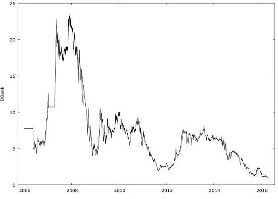
[image:8.595.237.512.292.489.2]

Figure 1 and Figure 2 are the share prices of Diamond and Fidelity Banks. Their movements appeared to fluctuate away from the common mean indicating the presence of stochastic nonstationarity.

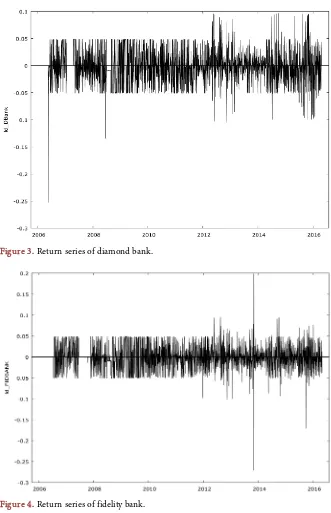
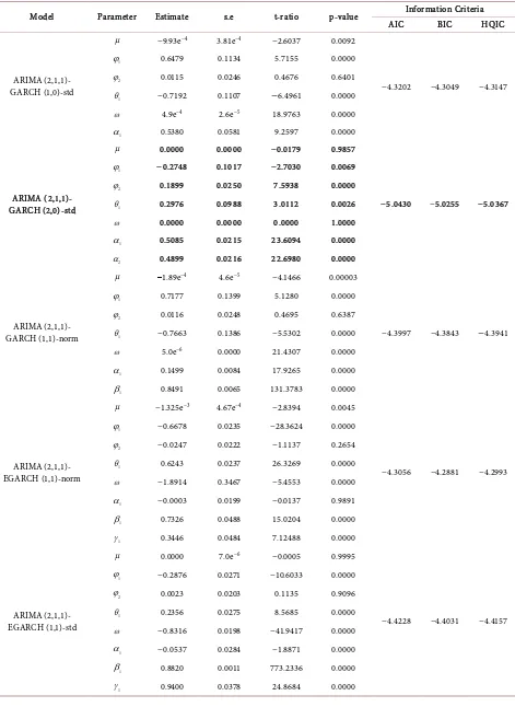
Figure 3 and Figure 4 are the returns series of the respective banks and are found to cluster around the common mean signifying stationarity.

[image:8.595.234.517.306.706.2]

Figure 1. Share price series of diamond bank.

[image:8.595.236.515.507.712.2]

(9)

[image:9.595.207.538.62.575.2]

DOI: 10.4236/am.2019.105024 341 Applied Mathematics Figure 3. Return series of diamond bank.

Figure 4. Return series of fidelity bank.

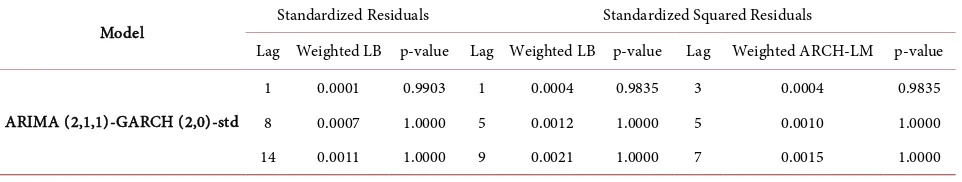
3.2. In-Sample Model Selection

(10)

[image:10.595.64.535.88.734.2]

DOI: 10.4236/am.2019.105024 342 Applied Mathematics Table 1. Estimation of Heteroscedastic models of return series of diamond bank.

Model Parameter Estimate s.e t-ratio p-value Information Criteria AIC BIC HQIC

ARIMA (2,1,1)- GARCH (1,0)-std

µ _−9.93e−4 _3.81e−4 _−2.6037 _0.0092

−4.3202 −4.3049 −4.3147 1

ϕ 0.6479 0.1134 5.7155 0.0000

2

ϕ _0.0115 _0.0246 _0.4676 _0.6401

1

θ −0.7192 0.1107 −6.4961 0.0000

ω 4.9e−4 _2.6e−5 _18.9763 _0.0000

1

α 0.5380 0.0581 9.2597 0.0000

ARIMA (2,1,1)- GARCH (2,0)-std

µ _0.0000 _0.0000 _−0.0179 _0.9857

−5.0430 −5.0255 −5.0367 1

ϕ −0.2748 0.1017 −2.7030 0.0069

2

ϕ _0.1899 _0.0250 _7.5938 _0.0000

1

θ 0.2976 0.0988 3.0112 0.0026

ω 0.0000 0.0000 0.0000 1.0000

1

α 0.5085 0.0215 23.6094 0.0000

2

α _0.4899 _0.0216 _22.6980 _0.0000

ARIMA (2,1,1)- GARCH (1,1)-norm

µ −_1.89e−4 _4.6e−5 _−4.1466 _0.00003

−4.3997 −4.3843 −4.3941 1

ϕ 0.7177 0.1399 5.1280 0.0000

2

ϕ 0.0116 0.0248 0.4695 0.6387

1

θ _−0.7663 _0.1386 _−5.5302 _0.0000

ω 5.0e−6 _0.0000 _21.4307 _0.0000

1

α _0.1499 _0.0084 _17.9265 _0.0000

1

β 0.8491 0.0065 131.3783 0.0000

ARIMA (2,1,1)- EGARCH (1,1)-norm

µ _−1.325e−3 _4.67e−4 _−2.8394 _0.0045

−4.3056 −4.2881 −4.2993 1

ϕ −0.6678 0.0235 −28.3624 0.0000

2

ϕ _−0.0247 _0.0222 _−1.1137 _0.2654

1

θ 0.6243 0.0237 26.3269 0.0000

ω −1.8914 0.3467 −5.4553 0.0000

1

α −0.0003 0.0199 −0.0137 0.9891

1

β 0.7326 0.0488 15.0204 0.0000

1

γ 0.3446 0.0484 7.12488 0.0000

ARIMA (2,1,1)- EGARCH (1,1)-std

µ _0.0000 _7.0e−6 _−0.0005 _0.9995

−4.4228 −4.4031 −4.4157 1

ϕ −0.2876 0.0271 −10.6033 0.0000

2

ϕ _0.0023 _0.0203 _0.1135 _0.9096

1

θ 0.2356 0.0275 8.5685 0.0000

ω −0.8316 0.0198 −41.9417 0.0000

1

α −0.0537 0.0284 −1.8871 0.0000

1

β _0.8820 _0.0011 _773.2336 _0.0000

1

(11)

Ljung-Box Q statistics at lags 1, 5 and 9 on standardized squared residuals and weighted Lagrange Multiplier statistics at lags 3, 5 and 7 are all greater than 5% level of significance [see Table 2]. That is to say, the hypotheses of no autocor-relation and no remaining ARCH effect are not rejected.

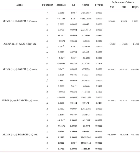
Also, for Fidelity Bank, ARIMA (1,1,0)-GARCH (1,0)-norm, ARIMA (1,1,0)-GARCH (1,0)-std, ARIMA (1,1,0)-GARCH (1,1)-norm, ARIMA (1,1,0)-EGARCH (1,1)-norm and ARIMA (1,1,0)-EGARCH (1,1)-std were con-sidered tentatively (Table 3). Based on smallest information criteria, ARIMA (1,1,0)-EGARCH (1,1)-std was chosen as the appropriate model. The selected model is adequate since all the p-values corresponding to weighted Ljung-Box Q statistics at lags 1, 2 and 5 on standardized residuals, weighted Ljung-Box Q sta-tistics at lags 1, 5 and 9 on standardized squared residuals and weighted La-grange Multiplier statistics at lags 3, 5 and 7 are greater than 5% level of signi-ficance [see Table 4]. That is to say, the null hypotheses of no autocorrelation and no ARCH effect are not rejected at 5% significance level.

3.3. Out-Of-Sample Forecasting Model Selection

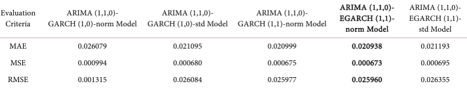
Here, the out-of-sample forecast evaluation criteria; MAE, MSE and RMSE for each of the models are considered for the series of the banks. It was found that ARIMA (2,1,1)-EGARCH (1,1)-norm and ARIMA (1,1,0)-EGARCH (1,1)-norm possessed the smallest out-of-sample forecast evaluation criteria (see Table 5 and Table 6). Hence, the most appropriate for the return series of the respective banks.

Based on our findings, the in-sample model selection procedure favoured ARIMA (2,1,1)-GARCH (2,0)-std and ARIMA (1,1,0)-EGARCH (1,1)-std model while the out-of-sample model selection sufficed the choice of ARIMA (2,1,1)-EGARCH (1,1)-norm and ARIMA (1,1,0)-EGARCH (1,1)-norm models for the banks considered. Majorly, it is discovered that in each of the models se-lected through in-sample criteria are ill-conditioned. For instance, the constant term of the variance equation, ω of ARIMA (2,1,1)-GARCH (2,0)-std is zero which actually violates the constraint condition that requires

ω

>0_{. The}

impli-cation is that, this model is not suitable for forecasting long-run variance as it would collapse at zero. Again, in EGARCH (1,1)-std, the stationarity condition which requires

∑

pj

β

j<1, is violated. The implication is that, forecasting

[image:11.595.59.540.638.729.2]

long-run variance using this model would not be realistic in that the variance

Table 2. Diagnostic checking for heteroscedastic models of return series of diamond bank.

Model Standardized Residuals Standardized Squared Residuals

Lag Weighted LB p-value Lag Weighted LB p-value Lag Weighted ARCH-LM p-value

ARIMA (2,1,1)-GARCH (2,0)-std

(12)

[image:12.595.60.535.90.611.2]

DOI: 10.4236/am.2019.105024 344 Applied Mathematics Table 3. Estimation of heteroscedastic models of return series of fidelity bank.

Model Parameter Estimate s.e t-ratio p-value Information Criteria AIC BIC HQIC

ARIMA (1,1,0)-GARCH (1,0)-norm

µ _0.0181 _2.0e−6 _7416.5857 _0.0000

9.5841 9.5929 9.5873 1

ϕ −0.1188 4.1e−5 _−2892.9449 _0.0000

ω 0.0000 0.0000 4.8845 0.0000

1

α _0.9755 _0.0004 _2331.4143 _0.0000

ARIMA (1,1,0)-GARCH (1,0)-std

µ −_8.0e−4 _0.0004 _−1.9660 _0.0493

−4.4395 −4.4286 −4.4356 1

ϕ −0.0671 0.0241 −2.7856 0.0053

ω 4.0e−4 _2.3e−5 _18.2910 _0.0000

1

α _0.6093 _0.0739 _8.2413 _0.0000

ARIMA (1,1,0)-GARCH (1,1)-norm

µ −_5.0e−4 _9.0e−5 _−56.1884 _0.0000

−4.5492 −4.5382 −4.5452 1

ϕ −0.0339 0.0225 −1.5108 0.1308

ω 5.0e−6 _0.0000 _67.9874 _0.0000

1

α _0.1528 _0.0105 _14.5331 _0.0000

1

β 0.8462 0.0088 95.5935 0.0000

ARIMA (1,1,0)-EGARCH (1,1)-norm

µ _0.0000 _2.0e−5 _−0.0004 _0.9997

−4.5912 −4.5781 −4.5865 1

ϕ _−0.0363 _0.0231 −1.5721 0.1159

ω −0.6564 0.0065 −101.1563 0.0000

1

α 0.0155 0.0164 0.9474 0.3434

1

β 0.9063 0.0007 1341.0781 0.0000

1

γ 0.4184 0.0107 38.9643 0.0000

ARIMA (1,1,0)-EGARCH (1,1)-std

µ −_4.0e−6 _0.0000 _−41.393 _0.0000

−5.1507 −5.1354 −5.1452 1

ϕ −0.1572 0.0029 −56.078 0.0000

ω 0.0141 0.0003 49.642 0.0000

1

α _1.1589 _{0.0001 12452.741} _0.0000

1

β 1.0000 1.0e−5 _84465.444 _0.0000

1

γ 1.1730 0.0001 11481.44 0.0000

Table 4. Diagnostic checking for Heteroscedastic models of return series of fidelity bank.

Model Standardized Residuals Standardized Squared Residuals

Lag Weighted LB p-value Lag Weighted LB p-value Lag Weighted ARCH-LM p-value

ARIMA (1,1,0)-EGARCH (1,1)-std

[image:12.595.58.539.641.731.2]

(13)

[image:13.595.56.544.89.180.2]

DOI: 10.4236/am.2019.105024 345 Applied Mathematics Table 5. Out-of-sample forecast evaluation criteria for diamond bank.

Evaluation

Criteria GARCH (1,0)-std Model ARIMA (2,1,1)- GARCH (2,0)-std Model ARIMA (2,1,1)- GARCH (1,1)-norm Model ARIMA (2,1,1)-

ARIMA (2,1,1)- EGARCH (1,1)- norm Model

ARIMA (2,1,1)- EGARCH (1,1)-

std Model MAE 0.019999 0.022278 0.020026 0.019986 0.020047 MSE 0.000629 0.000772 0.000634 0.000628 0.000636 RMSE 0.025084 0.027785 0.025179 0.025078 0.025218

Table 6. Out-of-sample forecast evaluation criteria for fidelity bank.

Evaluation

Criteria GARCH (1,0)-norm Model ARIMA (1,1,0)- GARCH (1,0)-std Model ARIMA (1,1,0)- GARCH (1,1)-norm Model ARIMA (1,1,0)-

ARIMA (1,1,0)- EGARCH (1,1)- norm Model

ARIMA (1,1,0)- EGARCH (1,1)-

std Model MAE 0.026079 0.021095 0.020999 0.020938 0.021193 MSE 0.000994 0.000680 0.000675 0.000673 0.000695 RMSE 0.001315 0.026084 0.025977 0.025960 0.026355

would converge at infinity. Moreover, the highly significance of the parameters of the models indicated that the models are over-fitted. Meanwhile, the models selected through out-of-sample criteria are characterized by non-significant pa-rameters yet possessed smallest predictive errors and problem associated with over-fitting is overcome. In particular, this study showed that the study of [28] can be improved by adopting out-of-sample forecasting procedure. Further-more, the study is in agreement with the works of [1], [2], [22] by supporting the choice of models based on smallest predictive errors.

4. Conclusion

In all, our study showed that out-of-sample model selection approach outper-formed the in-sample counterpart in describing the characterization of future observations without necessarily considering the choice of true model. The ma-jor strength of this study is in utilizing the advantage of combining both ARIMA and GARCH-type models to achieve forecast accuracy. The weakness of this study is in adopting larger samples of training data against smaller sample sizes for forecast evaluation, which is suitable for achieving the best fitting models. However, this weakness could be overcome by adopting smaller sample sizes of data for model formulation and larger samples for forecast evaluation in future study.

Conflicts of Interest

The authors declare no conflicts of interest regarding the publication of this paper.

References

[image:13.595.64.537.214.303.2]

(14)

Over-DOI: 10.4236/am.2019.105024 346 Applied Mathematics

view. IEEE Signal Processing Magazine, 21, 1-21. http://arXiv:1810.09583v1 [2] Leeb, H. (2008) Evaluation and Selection of Models for Out-of-Sample Prediction

when the Sample Size Is Small Relative to the Complexity of the Data-Generating Process. Bernoulli, 14, 661-690.https://doi.org/10.3150/08-BEJ127

[3] Sinharay, S. (2010) An Overview of Statistics in Education. In: Peterson, P., et al., Eds., International Encyclopedia of Education, 3rd Edition, Elsevier Ltd., Amster-dam, 1-11.https://doi.org/10.1016/B978-0-08-044894-7.01719-X

[4] Montgomeny, D.C., Jennings, C.L. and Kulahci, M. (2008) Introduction to Time Se-ries Analysis and Forecasting. John Wiley & Sons, Hoboken, 18-60.

[5] Wei, W.W.S. (2006) Time Series Analysis Univariate and Multivariate Methods. 2nd Edition, Addison Wesley, New York, 33-59.

[6] Akaike, H. (1973) A New Look at the Statistical Model Identification. IEEE Trans-actions on Automatic Control, 19, 716-723.

https://doi.org/10.1109/TAC.1974.1100705

[7] Schwarz, G. (1978) Estimating the Dimension of a Model. Annals of Statistics, 6, 461-464. https://www.jstor.org/stable/2958889

https://doi.org/10.1214/aos/1176344136

[8] Hannan, E. and Quinn, B. (1979) The Determination of the Order of an Au-to-Regression. Journal of Royal Statistical Society, Series B,41, 190-195.

https://www.jstor.org/stable/2985032

https://doi.org/10.1111/j.2517-6161.1979.tb01072.x

[9] Zou, H. and Yang, G. (2004) Combining Time Series Models for Forecasting. In-ternational Journal of Forecasting, 20, 69-84.

https://doi.org/10.1016/S0169-2070(03)00004-9

[10] Box, G.E.P., Jenkins, G.M. and Reinsel, G.C. (2008) Time Series Analysis: Forecast-ing and Control. 3rd Edition, John Wiley & Sons, Hoboken, 5-22.

https://doi.org/10.1002/9781118619193

[11] Bozdogan, H. (2000) Akaike’s Information Criteria and Recent Developments In-formation Complexity. Journal of Mathematical Psychology,44, 62-91.

https://doi.org/10.1006/jmps.1999.1277

[12] Wasserman, L. (2000) Bayesian Model Selection and Model Averaging. Journal of Mathematical Psychology,44, 92-107.https://doi.org/10.1006/jmps.1999.1278

[13] Myung, I.J. (2000) The Importance of Complexity in Model Selection. Journal of Mathematical Psychology,44, 190-204.https://doi.org/10.1006/jmps.1999.1283

[14] Zucchini, W. (2000) An Introduction to Model Selection. Journal of Mathematical Psychology,44, 41-61.https://doi.org/10.1006/jmps.1999.1276

[15] Pilatowska, M. (2011) Information and Prediction Criteria in Selecting the Fore-casting Model. Dynamic Econometric Models, 11, 21-40.

https://doi.org/10.12775/DEM.2011.002

[16] Chatfield, C. (2000) Time Series Forecasting. 5th Edition, Chapman and Hall CRC, New York.

[17] Moffat, I.U. and Akpan, E.A. (2014) Time Series Forecasting: A Tool for Out-Sample Model Selection and Evaluation. American Journal of Scientific and Industrial Research,5, 185-194.

[18] Mitchell, H. and Mokenzie, M.D. (2010) GARCH Model Selection Criteria. Quan-titative Finance, 3, 262-284. https://doi.org/10.1088/1469-7688/3/4/303

(15)

Selec-DOI: 10.4236/am.2019.105024 347 Applied Mathematics

tion. The European Journal of Finance, 9, 557-580. https://doi.org/10.1080/1351847021000029188

[20] Degiannakis, S. and Xekalaki, E. (2005) Predictability and Model Selection in the Context of ARCH Models. Journal of Applied Stochastic Models in Business and Industry, 21, 55-82.https://doi.org/10.1002/asmb.551

[21] Bal, C., Demir, S. and Aladag, C.H. (2016) A Comparison of Different Model Selec-tion Criteria for Forecasting EURO/USD Exchange Rates by Feed Forward Neural Network. International Journal of Computing, Communication and Instrumental-ism Engineering, 3, 271-275.https://doi.org/10.15242/IJCCIE.U0616010

[22] Psaradakis, Z., Sola, M., Spagnolo, F. and Spagnolo, N. (2009) Selecting Nonlinear Time Series Models Using Information Criteria. Journal of Time Series Analysis, 30, 369-394.https://doi.org/10.1111/j.1467-9892.2009.00614.x

[23] Pena, D. and Rodriguez, J. (2005) Detecting Nonlinearity in Time Series by Model Selection Criteria. International Journal of Forecasting, 21, 731-748.

https://doi.org/10.1016/j.ijforecast.2005.04.014

[24] Manzan, S. (2004) Model Selection for Non Linear Time Series. Empirical Econom-ics, 29, 901-920.https://doi.org/10.1007/s00181-004-0207-7

[25] Judd, K. and Mees, A. (1995) On Selecting Models for Nonlinear Time Series. Phy-sica D: Nonlinear Phenomena, 82, 426-444.

https://doi.org/10.1016/0167-2789(95)00050-E

[26] Liu, Y. and Enders, W. (2003) Out-of-Sample Forecasts and Nonlinear Model Selec-tion with an Example of the Term Structure of Interest Rates. Southern Economic Journal, 69, 520-540. https://www.jstor.org/stable/1061692

https://doi.org/10.2307/1061692

[27] Gabriel, A.S. (2012) Evaluating the Forecasting Performance of GARCH Models: Evidence from Romania. Precedia-Social and Behavioral Sciences, 62, 1006-1010. https://doi.org/10.1016/j.sbspro.2012.09.171

[28] Akpan, E.A., Lasisi, K.E. and Adamu, A. (2018) Modeling Heteroscedasticity in the Presence of Outliers in Discrete-Time Stochastic Series. Academic Journal of Ap-plied Mathematical Sciences, 4, 61-76.

[29] Akpan, E.A. and Moffat, I.U. (2017) Detection and Modeling of Asymmetric GARCH Effects in a Discrete-Time Series. International Journal of Statistics and Probability, 6, 111-119.https://doi.org/10.5539/ijsp.v6n6p111

[30] Akpan, E.A., Moffat, I.U. and Ekpo, N.B. (2016) Arma-Arch Modeling of the Re-turns of First Bank of Nigeria. European Scientific Journal, 12, 257-266.

https://doi.org/10.19044/esj.2016.v12n18p257

[31] Onwukwe, C.E., Samson, T.K. and Lipcsey, Z. (2014) Modeling and Forecasting Daily Returns Volatility of Nigerian Banks Stocks. European Scientific Journal, 10, 449-467.

[32] Arowolo, W.B. (2013) Predicting Stock Prices Returns Using GARCH Model. In-ternational Journal of Engineering and Science, 2, 32-37.

[33] Emenike, K.O. and Friday, A.S. (2012) Modeling Asymmetric Volatility in the Ni-gerian Stock Exchange. European Journal of Business and Management, 4, 52-59. [34] Akpan, E.A., Lasisi, K.E., Adamu, A. and Rann, H.B. (2019) Evaluation of Forecasts

Performance of ARIMA-GARCH-Type Models in the Light of Outliers. World

Scientific News, 119, 68-84.

(16)

DOI: 10.4236/am.2019.105024 348 Applied Mathematics https://doi.org/10.2307/1912773

[36] Francq, C. and Zakoian, J. (2010) GARCH Models: Structure, Statistical Inference and Financial Applications. John Wiley & Sons Ltd., Chichester, 19-220.

https://doi.org/10.1002/9780470670057

[37] Bollerslev, T. (1986) Generalized Autoregressive Conditional Heteroscedasticity. Econometrics, 31, 307-327.https://doi.org/10.1016/0304-4076(86)90063-1

[38] Tsay, R.S. (2010) Analysis of Financial Time Series. 3rd Edition, John Wiley & Sons Inc., New York, 97-140.https://doi.org/10.1002/9780470644560

[39] Nelson, D.B. (1991) Conditional Heteroscedasticity of Asset Returns. A New Ap-proach. Econometrica, 59, 347-370.https://doi.org/10.2307/2938260