Ceriotti, M. and Vasile, M. (2009) MGA trajectory planning with an
ACO-inspired algorithm. In: 60th International Astronautical Congress,
2009-10-12 - 2009-10-16, Daejeon, Korea. ,
This version is available at
https://strathprints.strath.ac.uk/20160/
Strathprints is designed to allow users to access the research output of the University of Strathclyde. Unless otherwise explicitly stated on the manuscript, Copyright © and Moral Rights for the papers on this site are retained by the individual authors and/or other copyright owners. Please check the manuscript for details of any other licences that may have been applied. You may not engage in further distribution of the material for any profitmaking activities or any commercial gain. You may freely distribute both the url (https://strathprints.strath.ac.uk/) and the content of this paper for research or private study, educational, or not-for-profit purposes without prior permission or charge.
Any correspondence concerning this service should be sent to the Strathprints administrator:
The Strathprints institutional repository (https://strathprints.strath.ac.uk) is a digital archive of University of Strathclyde research outputs. It has been developed to disseminate open access research outputs, expose data about those outputs, and enable the
Ceriotti, M. and Vasile, M. (2009) MGA trajectory planning with an ACO-inspired algorithm. In:
60th International Astronautical Congress, 12-16 October 2009, Daejeon, Korea.
http://
strathprints
.strath.ac.uk/
20160
/
Strathprints is designed to allow users to access the research output of the University
of Strathclyde. Copyright © and Moral Rights for the papers on this site are retained
by the individual authors and/or other copyright owners. You may not engage in
further distribution of the material for any profitmaking activities or any commercial
gain. You may freely distribute both the url (http://
strathprints
.strath.ac.uk) and the
content of this paper for research or study, educational, or not-for-profit purposes
without prior permission or charge. You may freely distribute the url
(http://
strathprints
.strath.ac.uk) of the Strathprints website.
IAC-09.C1.1.3
MGA TRAJECTORY PLANNING WITH AN ACO-INSPIRED ALGORITHM
Matteo Ceriotti
Department of Aerospace Engineering, University of Glasgow, Glasgow, United Kingdom [email protected]
Massimiliano Vasile
Department of Aerospace Engineering, University of Glasgow, Glasgow, United Kingdom [email protected]
ABSTRACT
Given a set of celestial bodies, the problem of finding an optimal sequence of gravity assist manoeuvres, deep space manoeuvres (DSM) and transfer arcs connecting two or more bodies in the set is combinatorial in nature. The number of possible paths grows exponentially with the number of celestial bodies. Therefore, the design of an optimal multiple gravity assist (MGA) trajectory is a NP-hard mixed combinatorial-continuous problem, and its automated solution would greatly improve the assessment of multiple alternative mission options in a shorter time. This work proposes to formulate the complete automated design of a multiple gravity assist trajectory as an autonomous planning and scheduling problem. The resulting scheduled plan will provide the planetary sequence for a multiple gravity assist trajectory and a good estimation of the optimality of the associated trajectories. We propose the use of a two-dimensional trajectory model in which pairs of celestial bodies are connected by transfer arcs containing one DSM. The problem of matching the position of the planet at the time of arrival is solved by varying the pericentre of the preceding swing-by, or the magnitude of the launch excess velocity, for the first arc. By using this model, for each departure date we can generate a full tree of possible transfers from departure to destination. Each leaf of the tree represents a planetary encounter and a possible way to reach that planet. An algorithm inspired by Ant Colony Optimization (ACO) is devised to explore the space of possible plans. The ants explore the tree from departure to destination adding one node at the time: every time an ant is at a node, a probability function is used to select one of the remaining feasible directions. This approach to automatic trajectory planning is applied to the design of optimal transfers to Saturn and among the Galilean moons of Jupiter, and solutions are compared to those found through traditional genetic-algorithm-based techniques.
FULL TEXT
INTRODUCTION
The complete automatic design of multiple gravity assist trajectories (MGA), that is the definition of an optimal sequence of planetary encounters and the definition of one or more locally optimal trajectories for each sequence, has been approached with several different techniques. All of them can be classified in two main categories: two level approaches and integrated approaches.
Two-level approaches split the problem into two problems which lay at two different levels: one sub-problem is to find the optimal sequence of planetary encounters; the other is to find an optimal trajectory for that sequence. Two-level approaches define the planetary sequence independently of the trajectory itself. Once the sequence (or a set of promising sequences) has been selected, then the optimal trajectory can be searched for within the set of selected sequences only [1]. Simplified, low fidelity, models for representing the trajectory [2] are used at the first level: this allows for a quick assessment of many sequences, if not all. At the second level, a full model is used to optimize the trajectory. Each sequence is represented by a string of integer numbers, while the associated trajectory is represented with a string of real
and integer numbers defining the time and the characteristics of the events occurring along the trajectory (e.g. launch, deep space manoeuvre, arrival at a celestial body, number of revolutions around the Sun, etc.). Therefore, for each sequence, there is an infinite variety of possible trajectories.
The issue with two-level approaches is that it is difficult to assess the optimality of a given planetary sequence without an exhaustive search for all possible trajectories associated with that sequence. Unfortunately, finding an optimal trajectory is a very difficult global optimisation problem in itself. This, combined with the fact that usually there exist a very high number of sequences for a given transfer problem, requires a considerable computational effort. The computational cost can be reduced by discarding non-promising sequences. However, if the low-fidelity model is not accurate enough, either some good sequences are discarded, or many of the retained ones can result to be actually not interesting.
problem is known in literature as a hybrid optimization problem [4]. The main difficulty with integrated approaches is that a variation of even a single celestial body in the sequence corresponds to a substantially different set of trajectories. In addition, a variation of the length of the sequence implies varying the number of legs of the trajectory, and thus the total length of the solution vector.
The automatic design of a trajectory with discrete events was recently formulated as a hybrid optimal control problem [5], and a solution was proposed by Conway et al. [6] with a two level approach based on genetic algorithms.
Here we propose to formulate the complete automated design of a multiple gravity assist trajectory as an autonomous planning and scheduling problem. The resulting scheduled plan will provide the planetary sequence for a multiple gravity assist trajectory and a good estimation of the optimality of the associated trajectories.
Although the proposed method can fall in the category of the integrated approaches, the scheduling and the planning of the events are separated at two different levels. A specific MGA trajectory model was developed to automatically schedule the events, if a plan is available, and to provide a good estimation of the feasibility and quality of a trajectory. A novel algorithm, partially inspired by the Ant Colony Optimization (ACO) paradigm [7], was devised to explore the space of possible plans. ACO was originally created to solve the Travelling Salesman Problem [8], and later successfully applied to a number of other discrete optimisation problems. Here the original idea behind ACO was elaborated to solve the planning problem associated to the design of MGA trajectories. In the literature, some ACO-derived meta-heuristics exist for the specific solution of different scheduling problems. In particular, Merkle et al. [9] proposed to apply ACO to the solution of the Resource-Constrained Project Scheduling Problem, while Blum, in his work [10], suggested the hybridization of Ant Colony Optimization with a probabilistic version of Beam Search for the solution of the Open Shop Scheduling problem.
In this paper, at first we will present the trajectory model and the integrated scheduling of the events, then the novel ACO-based algorithm and how the plan is constructed. Finally, three case studies will demonstrate the effectiveness of the proposed approach at solving known space trajectory design problems.
TRAJECTORY MODEL
The trajectory model is devised having in mind the planning and scheduling process and the planning algorithm fully exploits its characteristics.
The model is based on a two-dimensional linked-conic approximation of the trajectory and planar orbits of the planets. The trajectory is composed of a sequence of planar conic arcs linked together through discrete,
instantaneous events. In particular, the sequence is continuous in position and piecewise continuous in velocity, i.e. each event introduces a discontinuity in the velocity of the spacecraft but not in its position. The discrete events can be: launch, deep space manoeuvre (DSM), swing-by, and brake.
A final assumption of the present implementation is that all the orbits of both spacecraft and celestial bodies are direct, thus no retrograde orbits are allowed.
In summary, the proposed trajectory model is composed of: a launch from the departure celestial body; a series of deep space flight legs connected through gravity assist manoeuvres (modelled through a linked-conic approximation); an arrival at a target celestial body. Each one of these basic components will be explained in the following.
Launch
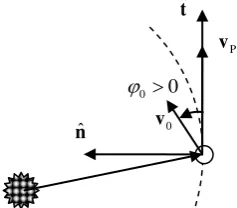
The launch event is modelled as an instantaneous change of the velocity of the spacecraft with respect to the departure planet. The velocity change is given in terms of modulus v0 (which depends on the capabilities of the launcher) and in-plane direction, specified through the angle 0, measured counter clockwise with respect to the planet’s orbital velocity vector vP at time of launch t0.
0
t and 0 are free parameters of the model, while launch
velocity modulus v0 will be used to target the next
planetary encounter and solve the phasing problem, as explained later.
Fig. 1: Geometry of the launch, and convention for launch angle.
Swing-by
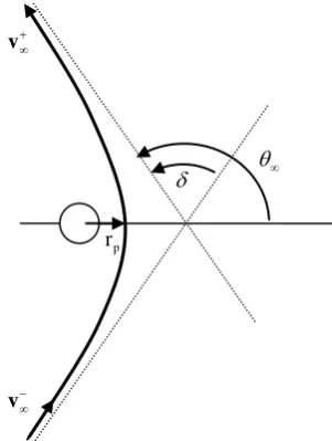
Gravity assist manoeuvres, or swing-bys, are modelled as instantaneous changes of the velocity vector of the spacecraft due solely to the gravity field of the planet. Given the relative velocity vector v before the swing-by, the physical properties of unperturbed hyperbolic orbital motion prescribe that v v v, which means that the modulus of the outgoing velocity v at infinity is known. Its direction can be computed considering the anomaly of the outgoing asymptote (see Fig. 2):
2
arccos P p
P p
r
v r
. (1)
P
v
0
v
0 0
ˆ
t
ˆ
[image:4.612.379.498.421.525.2]Here, P is the gravity constant of the planet, and r is p
the radius of the pericentre of the hyperbola. The value of
p
r can be used to control the magnitude of the deflection angle
2
of the incoming velocity and is limited to be above the radius of the planet, RP, to avoida collision, or to be above the atmosphere to avoid a re-entry. The direction of deflection is determined using a signed radius of pericentre r , such that ps rp rps and
sgn rps 2
.
[image:5.612.91.242.276.476.2]Once is computed, the relative outgoing velocity is calculated by rotating v in the plane of an angle . As for the launch velocity magnitude, the radius of pericentre r is tuned to meet the terminal conditions of ps the transfer leg following the swing-by.
Fig. 2: Geometry of the swing-by. Deep space flight leg
Each deep space flight leg starts at a departure planet Pi
and ends at an arrival planet Pi1, and is made of two
conic arcs linked at a point Mi. If the leg contains a deep
space manoeuvre, this is applied in this point, and it produces an instantaneous change in the heliocentric velocity vector of the spacecraft, due to an ignition of the engines. In this model, we assume that the DSM is performed either at the apocentre or pericentre of the conic arc preceding the manoeuvre. In addition, the change in velocity is tangential to that arc.
For clarity, in the remainder of this section, we neglect the subscript index i of the leg in all the variables.
First arc
Let us assume that the spacecraft is at a given planet P1
at time t1. Its position coincides with that of the planet,
which is known from the 2D ephemeris. The heliocentric
velocity of the spacecraft, instead, depends on the preceding launch or swing-by event.
If the transfer leg contains a DSM, the first step is to find the position M and time tDSM of the deep space manoeuvre. The position can either be the pericentre or the apocentre, according to a binary parameter fp a/ . The true anomaly of the DSM is given by
/
0 0
1
DSM p a
DSM
f
.
The time of the DSM tDSM is found by using the time
law. The parameter nrev,1 is used to count the number of full revolutions before the deep space manoeuvre. At M, the DSM is applied tangentially, being the free parameter mDSM the magnitude and direction of the
DSM: if mDSM is positive, the thrust is along the velocity
of the spacecraft, otherwise it is against the velocity of the spacecraft. The complete state of the spacecraft at the beginning of the second arc is thus fully determined. If the leg does not contain any DSM, i.e. mDSM 0, the first arc is propagated up to a fictitious point M, defined by adding an angle to the initial true anomaly of the spacecraft. The quantity is a small angular
displacement, larger than the machine numerical precision, but small enough to allow for the modelling of very short transfer legs. For this work, 0.3 rad was chosen. The time tM at M is found by solving again the
time law. In this case, parameters fp a/ and nrev,1 are not
used.
Second arc
The second arc starts at point M and is propagated until the intersection of the orbit of planet P2. Given the orbital parameters of the spacecraft at M, and the orbital parameters of planet P2, the task is to find the
intersection between the two coplanar orbits. If there are no intersections, the leg is unfeasible, and the initial conditions of the leg, or its parameters, have to be changed. Otherwise, one of the two intersections is selected according to the binary parameter f1/ 2: let us
call int, the true anomalies of the selected intersection,
respectively along the orbit of the spacecraft and of the planet. From int, the time tint at which the spacecraft
intersects P2’s orbit can be computed with the time law, and considering the integer parameter nrev,2 counting the
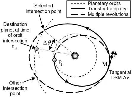
number of full revolutions between the point M and the orbital intersection. Fig. 3 illustrates a complete leg, including a DSM. The figure highlights that the orbital intersection does not imply, in general, that the planet is at the intersection point at the correct time. This issue will be addressed in the following paragraph.
v
v
p
Fig. 3: Representation of a complete leg, starting from P1
with either a swing-by or launch, with a DSM and possibly multiple revolutions. The phasing problem at P2 is not solved, as P2 at the time of intersection
is not at the intersection point.
Solution of the Phasing Problem
In order to perform a gravity assist manoeuvre or a planetary capture, the terminal position of the spacecraft has to match that of the planet. However, at intersection time tint, planet P2 is at true anomaly
2
P
, which is
generally different from . The time of intersection is a function of the states at the beginning of the leg, which ultimately depend on v0 or r depending on the starting ps
event. Therefore, if we introduce the symbol , such that
ps
r
if swing-by, or v0 if launch.
The true anomalies of the intersection point and of the planet can be expressed as
and
2
P
. Matching the position of the planet with that of the intersection point at time tint (also known as the phasing problem),
then, translates into finding a value *
=
that satisfies the equation (see Fig. 4):
2
* * *
0
P
(2)
Fig. 4: The phasing problem consists of finding such that the target planet P2 is at the orbital intersection
point at the correct time. This is done by finding the zero of the difference in true anomalies .
Fig. 5 (a) and (b) represent the function
for different transfer cases. The non-resonant case depicted in Fig. 5 (a) shows that the function
is continuous, smooth and monotonic over the range of interest of . Hence, the phasing problem has only one solution. This solution can be found with a simple Newton-Raphson method in one dimension. However, when a resonant transfer is considered, as in Fig. 5 (b),
is discontinuous and multiple zeros exist. Each zero corresponds to a different resonance with the planet (and of course a different transfer time). Since there is no easy way, at a given transfer, to prefer one value of over another, all the solutions need to be retained for the evaluation of the following transfers.
In ACO-MGA, the search for the zeros of the function
is performed with the Brent method. A set of starting points, defining multiple intervals for the bisection method, needs to be provided to initialize the Brent method and are specified case by case.
Note that in the examples in Fig. 5, the parameter is the launch excess velocity v0. It is possible to show that
the same behaviour of
holds for a leg starting with a swing-by (i.e. rps).a)
0 1 2 3 4 5 6 7
-0.4 -0.2 0 0.2 0.4 0.6 0.8 1 1.2 1.4 1.6
v 0
b)
2 3 4 5 6 7 8
-4 -3 -2 -1 0 1 2 3 4
v 0
Fig. 5:
v0 for: (a) Earth to Venus leg followinglaunch from Earth. (b) Earth to Earth leg following launch from Earth.
Selected intersection point
Destination planet at time
of orbit intersection
Other intersection
point
Tangential
DSM v 1
P
2
P
M
Planetary orbits Transfer trajectory Multiple revolutions
int
t
Planet position at intersection time tint
Selected intersection point
Spacecraft orbit
2P
2
[image:6.612.317.550.60.710.2] [image:6.612.329.538.367.694.2] [image:6.612.53.289.407.676.2]Complete trajectory
A complete trajectory is made of a sequence of transfer legs connecting nP1 celestial bodies P P0, ,1PnP.
The trajectory starts from P0 at time t0 with a launch event characterized by a departure angle 0. The first leg
goes from P0 to P1, then a number of swing-bys and interplanetary legs follow, until the final planet
P
n
P . Thus, a complete trajectory with nP1 planets has nP legs, and nP1 swing-bys.
The solution of Eq. (2) provides a complete scheduling of the trajectory given the initial time t0 and the five parameters mDSM,nrev,1,nrev,2,fp a/ ,f1/ 2i for every leg
0,..., P 1 i n .
Since these five parameters fully characterize all possible legs from a planet Pi to a planet Pi1, they are said to
define a type of transfer. Conversely, because of the multiplicity of the zeros of Eq. (2), each type of transfer corresponds to a set of trajectories.
Hence, assigning a value to t0, 0, Pi, PnP,
,1 ,2 / 1/ 2
, , , ,
DSM rev rev p a i
m n n f f
for i0,...,nP1 creates a plan, or solution, which is a tree structure in which every branch, from root to leaves, is a trajectory. Each trajectory is characterised by a different combination of
* 0
v and rp* for each leg.
The entire tree is a complete set of trajectories from P0 to
P
n
P and represents a solution of the MGA trajectory planning problem. Thus, a plan is fully defined by assigning a value to the parameters in Table 1 for all
0,..., P 1 i n .
An algorithm keeps track of all the trajectories in the tree, and yields a list containing all the possible conditions of arrival at the last reachable planet. If no trajectory in the set associated to leg i satisfies the phasing problem, then planet i1 cannot be reached and the algorithm terminates. A partial or incomplete solution is the set of parameters sufficient to describe a solution up to leg i. Furthermore, if no solution to the phasing problem exists at leg i, the plan is broken and the solution is said to be infeasible at leg i. Furthermore, an upper bound on the time of flight of the entire trajectory, or of some legs, is introduced. Trajectories that exceed the total or partial time of flight constraint are discarded from the list. The information of infeasibility at a given transfer will be used to fill in a taboo list of broken or incomplete solutions.
For each of the trajectories found, the model computes: the sum of all the deep space manoeuvres, or total v and the launch excess velocity, v0; the relative velocity
at the last planet, v; the total time of flight of the trajectory, T. The objective value of the trajectory
depends on the problem and it is usually a function of these values.
The whole model was implemented in ANSI C and compiled as a MEX-file for interfacing with MATLAB.
Table 1: Description of the free design variables defining a solution according to the proposed 2D model. Description Variables Planetary sequence P P0, ,1PnP
Departure time t0
Departure angle 0
Types of transfer for i0,,nP1
,1 ,2 / 1/ 2
, , , ,
DSM rev rev p a i
m n n f f
THE ACO-MGA ALGORITHM
The model described in the previous section yields a set of scheduled trajectories provided that a complete or partial plan is available. In this section, we present an optimization procedure, based on the ant colony optimization paradigm, to explore the space of possible plans.
At first, the continuous space of the real parameters t0, 0
and mDSM i is reduced to a finite set of states. Then, the optimization algorithm, called ACO-MGA in the following, operates a search in the finite space of possible values for the design parameters. A complete description of the algorithm ACO-MGA follows.
Solution coding
In ACO-MGA, a solution is coded through a string of discrete values assigned to the parameters. However, the set of parameters discussed before is inhomogeneous, as it is made of real, integer and binary variables. In particular, t0, 0 and mDSM i are real continuous
variables and need to be properly discretised. In the present implementation of ACO-MGA, the values of the departure date t0 and the departure angle 0, are assumed to be pre-assigned and therefore the two parameters are removed from the list of the variables. The rationale behind this choice is that, although the launch date has a great impact on the resulting trajectory, if an algorithm exists that is able to efficiently generate a complete plan for a given launch date, a systematic search can be performed along the launch window, with a given time step. We will show in the following that a systematic search is feasible. The angle 0 on the other
hand can very often be estimated depending on the mission [1].
Using the additional assumptions on t0, 0, and fixing 0
P , each solution can be coded using a vector s of positive integers. The vector has 2nlegs components. Each
the identification number of the target planet for the corresponding leg according to the following procedure: an ordered list qP i, containing all the planets available as a target for each leg i is predefined (and fixed); then, if
2i 1 1
ks , the target planet is the kth entry in the list
, P i
q , i.e. qP i k,( , ).
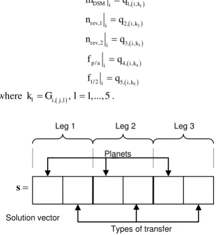
The second element of the pair is the row index of a matrix Gi containing all possible combinations of indexes identifying the elements of the five sets:
1,i, 2,i, 3,i, 4,i, 5,i
q q q q q . These sets contain the possible values for each one of the five parameters identifying the type of transfer at leg i. Thus, each row of Gi is a vector representing a different type of transfer. The parameters for the jth type of transfer for the ith leg can be obtained as follows:
1
2
3
4
5
1, , ,1 2, , ,2 3, , / 4, , 1/ 2 5, ,
DSMi i k rev i i k rev i i k p ai i k
i k i
m q
n q
n q
f q
f q
[image:8.612.59.275.264.495.2]where klGi, j l, ,l1,...,5.
Fig. 6: Solution vector s for coding a three-leg solution. The taboo and feasible lists
A transfer from planet Pi to planet Pi1 can be feasible or
unfeasible, for the same set of parameters, depending on all the preceding legs from 1 to
i1
. For this reason, when an infeasible leg is generated, it is necessary to store the path that led to that infeasible leg. Thus, all the parameters characterising the partial solution up to Pi1are stored in a taboo list.
In particular, if the problem involves nP legs, then the
same number of taboo lists are used. The taboo list of leg i contains all the partial solutions which are unfeasible at leg i (but feasible for legs 1i1). Each taboo list is stored in a matrix, which has an arbitrary number of rows and 2i columns.
Dual to the list of taboo partial solutions, the feasible list stores all the solutions, which are completely feasible, i.e.
reach
P
n
P . This is once more a matrix with an arbitrary number of rows and 2n columns. P
Since each solution contained in the feasible list is complete, then it is possible to associate an objective value to each one of them. A scalar value can be computed identifying the value of the trajectories. In the following test cases, we will use, as objective value, the v and a combination of v and T. Note that, since, in general, there is more than one trajectory for a given solution (i.e. for a given set of free design variables), the objective value of a solution is given by the best trajectory value.
Search engine
The search space is organised as an acyclic oriented tree. Each branch of the tree represents a leg of the problem, while each node (or leave) represents a different destination planet and type of transfer. A population of virtual ants are dispatched to explore the tree, searching for an optimal solution.
The search runs for a given number of iterations niter max, ,
or until a maximum number of objective function evaluations neval max, has been reached. An evaluation is a
call to the model, in order to compute the objective value associated to a given solution.
Algorithm 1 illustrates the main iteration loop. Each iteration consists of two steps: first, a solution generation step, and then a solution evaluation step. In the former step, the ants incrementally compose a set of solution vectors, while the latter invokes the trajectory model to assess the feasibility and the objective value of each generated solution. When the main loop of the search stops, the feasible list contains all the solutions, which were found feasible, with their corresponding objective value. The solutions are then sorted according to their objective value.
Algorithm 1: Main ACO-MGA search engine. 1 : While niter niter max, neval neval max, , Do 2 : For each ant k1m
3 : sGenerate planetary sequence 4 : sGenerate types of transfers 5 : If s is not discarded, S S
s6 : End For
7 : Evaluate all solutions in S
8 : Update feasible list and taboo lists 9 : Update niter,neval
10 : End Do
11 : Sort feasible list according to y.
Solution generation
The tree is simultaneously explored, from root to leaves, by m ants. At each iteration, each one of the m ants explores the tree independently of the others, but taking into account the information collected by all the ants at
Leg 1 Leg 2
Types of transfer Planets
Leg 3
Solution vector
the previous iterations, through the feasible list and the taboo lists. As an ant moves along a branch, it progressively composes a complete solution. At first, each ant assigns a value to the odd entries of the solution vector, i.e. composes the sequence of planetary encounters, then it assigns a value to the even entries of the solution vector, i.e. the parameters defining the type of transfer for each legs.
Planetary sequence generation
Each ant composes a solution adding one planet at the time. As the departure planet is given, the ant has only to choose the destination planet for each leg. The choice is made probabilistically by picking from the list qP i, . The
selection depends on the discrete probability distribution vector dP i, (one for every leg) which contains the
probability associated to each body in qP i, . Every time
an ant is at leg i, the probability distribution vector is reset to dP i,
1 1 1
T, i.e. all the planets have equal probability to be chosen, and the ant sweeps the entire list qP i, substituting the identification number of each element in qP i, into the ith
odd component of the partial solution vector s. Then, the feasible list is searched, for all the solutions which have a (partial) planetary sequence which matches the one in s. Say that the jth element of qP i, is added to s, and the resulting
partial sequence in s matches the partial sequence of the lth solution in the feasible lists, then the probability dP i j, , associated to the jth element of qP i, is increased as
follows:
, , , ,
1
planet P i j P i j
l
d d w
y
(3)
The amount of probability which is added depends on the objective value yl of the matching solution in the feasible list, and on the weight wplanet. Thus, the
probability of choosing the jth planet increases according to how many times it generates a promising sequence (leading to a feasible solution), to the value of the feasible solution itself, and to the parameter wplanet.
This mechanism is analogous to the pheromone deposition of standard ACO and aims at driving the search of the ants toward planetary sequences, which previously led to good solutions. In fact, those planets which generate (partial) sequences that appear either frequently in the feasible list, or rarely, but with low objective function are selected with higher probability. On the other hand, the probability of selecting other planets remains positive, such that one or more ants can probabilistically choose a planet that generates an undiscovered sequence. Note that, if the feasible list is empty, then all the planets have the same probability to be selected.
The parameter wplanet controls the learning rate of the
ants. A low value of wplanet will make the term wplanet yl
small, and thus the probability distribution will not change much, even if the solution appears repeatedly in the feasible list, or with low values of y. Thus, a relatively low value of wplanet will favour a global
exploration of the search space, while a high value of
planet
w will greatly increase the probability of choosing a planet which led to a feasible sequence. If the value of
planet
w is high enough with respect to a reference objective value, then the ant will preferably choose a feasible sequence, rather than trying a new one, which has not proven to be feasible. For these reasons, we can say that low values of wplanet will favour local
exploration of planetary sequences.
The procedure iterates for all the legs of the problem, and for all the ants. At the end, all the odd entries of the temporary solution s contain a target planet and the planetary sequence is complete. The next step is to find the type of transfers for each leg, thus filling the even entries of s and complete the solution.
Type of transfer generation
Once an ant has filled in the odd components of a solution s, it proceeds assigning values to the even components. Similarly to the planet sequence generation, for each transfer all the available types of transfer are assigned, one at the time, to the solution s. A vector s for which a value is assigned to both the odd and even components up to leg i represents a partial solution. Similarly to before, a vector dt i, contains the probability
distribution associated to the rows of the matrix Gi (i.e.
to each type of transfer).
For each new partial solution, the taboo list is first checked. If the partial solution appears in the taboo list, then it means that this solution will be infeasible, regardless of the way it is completed. The probability of the type of transfer associated to that sequence is set to zero, to avoid future selection of that type of transfer. If the partial solutions does not appear in the taboo list, the feasible list is searched for any matching partial solution. For every match found, the probability distribution for that type of transfer is modified as follows:
, , , ,
1
type t i j t i j
l
d d w
y
(4)
Where the weight wtype is introduced with analogous
meaning to wplanet. In fact, the higher the coefficient, the
higher the chances that solutions similar to the feasible ones are generated. Conversely, a low value of wtype will favour the selection of sequences with a different type of transfer, thus increasing the random exploration of the whole solution space.
probability distribution dt i, will be full of zeros. As a
consequence, the solution s (which can be partial or complete) is discarded, and the ant can stop its exploration of that branch of the tree. At the end of the solution generation step, the solution s is either discarded or completed. Once all the ants have completed their exploration, the result is a number of solutions (less than or equal to the number of ants m) to be evaluated. Solution evaluation
Once a set of solutions S has been generated by the ants, each solution has to be evaluated to assess its feasibility and its objective value. This is done by calling the trajectory model.
Solutions in S are evaluated one by one, by means of the model presented before. The trajectory model can be seen as a function which takes a solution vector s as an input, together with t0,0,P0, and gives as an output either an
objective value y (if the solution is feasible) or the leg lu at which the solution becomes unfeasible. If the solution is feasible, it is stored in the feasible list and lu 0, otherwise it is stored in the lu
th
taboo list.
CASE STUDIES
The proposed optimisation method was applied to two case studies inspired by the Laplace [11] and Cassini [12] missions, the former of which currently under preliminary study by ESA, NASA and JAXA.
ACO-MGA was tested against genetic algorithms, which are known to perform well on these kinds of problems. In particular, it was chosen to use the genetic algorithm implemented in MATLAB® within the Genetic Algorithm and Direct Search Toolbox™ (GATBX), and the Non-dominated Sorting Genetic Algorithm (NSGA-II) [13]. Settings for all the optimisers will be specified for each test case. While NSGA-II can deal with discrete variables, GATBX only uses real variables: a wrapper of the objective function was coded to round the continuous solution vector to the closest integer.
Due to the stochastic nature of the methods involved in the comparative tests, all the algorithms were run for 100 times. The performance index used to compare the ACO-MGA against the other global optimisers is the success rate: according to the theory developed in [14], 100 repetitions give an error in the determination for the exact success rate of less than 6%.
Some preliminary tests showed that the best performances of ACO-MGA are achieved if the algorithm is run in 2 steps, using different sets of parameters. In particular, in the first step, the weights
,
planet type
w w are set to 0: remembering Eq. (3) this choice translates into an initial pure random search. In the second step, weights are set to non-null values, to explore around the feasible solutions found.
The values of wplanet,wtype are set such that:
,
planet type
w w w y (5) where y is the expected minimum value for the objective function. In this way, choosing for example
1
w , a 1 is added to the probability of a given element every time a matching solution with objective y appears in the feasible list. The value of probability is higher if the objective value of the matching feasible solution is lower.
This two-step procedure can be explained in the following way. The first step allows a random sampling of the solution space, with the aim of finding a good number of feasible solutions. This is done to prevent the algorithm to stagnate around the first feasible solution found. The second step intensifies the search around the feasible solutions which were found at step one. Because of Eqs. (3) and (4), feasible solutions with low objective value are likely to be investigated further. In addition, the random component in the process does not forbid to keep exploring the rest of the search space.
The test cases were run on an Intel® Pentium® 4 3 GHz machine running Microsoft® Windows® XP.
Laplace case study
In this mission, the spacecraft reaches the sphere of influence of Jupiter after an interplanetary flight, and exploits a swing-by of Ganymede to get captured into the Jovian system. At this point, multiple swing-bys of Ganymede and Callisto are used to reduce the relative velocity to Callisto v, in order to be captured by the Moon and start the scientific phase.
The problem under consideration relates to the second part of the transfer: we assume that the interplanetary trajectory has been already optimised, including the first Ganymede gravity assist. The resulting orbit is a 3:1 resonance (spacecraft:planet) with Ganymede. The problem is to find the sequence of additional swing-bys, starting from the second one of Ganymede, to reach Callisto with low v.
For tackling this problem with ACO-MGA, a launch is simulated from Ganymede, and the initial conditions and type of transfer for the first leg (GG) are fixed. The other legs, instead, have free parameters to be optimised. The date of the first Ganymede swing-by is
0 9309.8 d, MJD2000
t , corresponding to 28th June 2025, where the spacecraft leaves the planet with an angle 0 1.2471rad. For defining the first leg according
to the design, the following set of parameters is considered:
,11,1 2,1 3,1 4,1 5,1
Ganymede 0 ; 0 ; 1
P
q
q q
q q
q
,11 2,1 rev
n q and fp a/ 1q4,1 are not influent. These
settings lead to a departure velocity from Ganymede of
0 5.1 km/s
v , as required.
Three free legs are added to problem. For the first two, the algorithm can choose to target Ganymede or Callisto, while for the third and last, the target must be Callisto:
, 1,
2, 3,
4, 5,
Ganymede, Callisto 10, 0,10 m/s 2,3 :
0 ; 0,1, 2,3 0,1 ; 0,1
P i i
i i
i i
i
q
q
q q
q q
,4 1,4
2,4 3,4
4,4 5,4
Callisto ; 10, 0,10 m/s 0 ; 0,1, 2,3
0,1 ; 0,1
P
q q
q q
q q
Small corrective DSM manoeuvres of 10 m/s can be used, and up to 3 complete revolutions can be performed. The number of revolutions is entirely controlled by the parameter nrev,2iq3,i. In general, there is no easy way
to identify whether the first or the second orbital intersection is the best one, so the binary parameter f1/ 2 i was left free to be chosen by the ants.
The radius of pericentre of the swing-bys is bounded between 1 and 3 radii RP of the body.
The total time of flight was limited to a maximum of 100 days and the objective function for a complete solution is the v at the final encounter with Callisto.
The average time for evaluating one solution (finding all the trajectories that generates) of this test case is 30.34 ms, and there are 9216 distinct solutions. Thus, a systematic approach, scanning all the solutions, would require 4.66 min.
All the optimisers were run for up to 600 function evaluations. GATBX and NSGA-II were run with the settings shown in Table 2. In addition, the initial population of GATBX is spread in the whole domain. Since the size of the population is very important for genetic-based algorithms, and it can affect the results significantly, this case study was also run 100 times with different sizes of the population (maintaining the predefined number of total function evaluations by varying the number of generations accordingly). For NSGA-II, it resulted that there was no noticeable change in the quality of the results over 100 runs. This is related to the fact that NSGA-II is not completely converging with only 600 function evaluations.
For GATBX, instead, results were changing significantly, and the settings leading to the best solutions were used. The parameters for ACO-MGA were tuned by trial and error, running the same test case for different values of the weights, the number of ants and the number of iterations. The best results were obtained with the following settings. 10 ants were used, with a first optimisation step with 30 iterations and wplanet,wtype0,
followed by a second step of 30 more iterations with , 20 3 km/s
planet type
w w . Because of the normalisation shown in Eq. (5), the weight values appear to have general validity, and can be applied also to other transfer problems, as will be shown in the next case study. Results in the form of statistical parameters over the 100 runs are presented in Table 3. All the algorithms found at least one feasible solution in every run. The value of 2 km/s as a target value for the v has been chosen to compute the success rate according to the procedure proposed in [15].
The results in Table 3 point out that, while all the algorithms find feasible solutions in all the runs, the quality of the solution is much better for ACO-MGA. Moreover, GATBX found a good solution only in 31% of the runs, and NSGA-II in 39%. ACO-MGA, instead, found a good solution in 62% of the runs.
The time for one ACO-MGA run is about 8 min. The simplicity of the test case, together with the implementation of ACO-MGA in a high-level language like MATLAB, makes the use of an optimisation method slower than the systematic scan of the whole solution space. Note that this will not happen in the more complex Cassini test case.
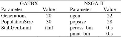
Table 2: Parameters of GATBX and NSGA-II for the Laplace test case.
GATBX NSGA-II
[image:11.612.326.557.375.446.2]Parameter Value Parameter Value Generations 20 ngen 22 PopulationSize 30 popsize 28 StallGenLimit +Inf pcross_bin 0.5 pmut_bin 0.5
Table 3: Comparison of the performances of ACO-MGA, GATBX, NSGA-II over 100 runs for the Laplace problem.
Average best value, km/s
% runs < 2 km/s
% feasible runs ACO-MGA 2.0141 62% 100% GATBX 2.34 31% 100% NSGA-II 2.1074 39% 100%
The reference solution for this problem, as chosen by ESA during a preliminary study, was re-optimised using a full 3D model with 1 free deep space manoeuvre per leg [16], and minimising the v : the resulting trajectory is represented in Fig. 7 (a), starting from the second swing-by of Ganymede. The sequence for this solution is GGCGC, and the objective value, i.e. the final relative velocity, is v 1.96 km/s. The solution is practically ballistic.
[image:11.612.327.556.492.551.2]solution with the re-optimised 3D solution. The similarity of the time of flights of each leg remarks that the two solutions are the same. Slight differences are due to the different models, and mainly to the changes of inclination that are needed in the 3D solution.
Note that the solution chosen by ESA, and used here as a comparison, is not the best from the point of view of the arrival velocity. In fact, this solution was chosen by ESA following a trade off, taking into account not only the v, but also the presence of DSMs, the total time of flight, the radiation dose, and the arrival velocity vector at Callisto.
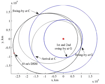
Solutions with lower v exist, and in fact were found by ACO-MGA. The best solution found has v1.71 km/s, and corresponds to the trajectory plotted in Fig. 8. The swing-by sequence is the same, GGCGC, but the total time of flight is much longer (92 days), since one leg performs 1 full revolution and another one 2 full revolutions. Also, a DSM of 10 m/s is used.
-2.5 -2 -1.5 -1 -0.5 0 0.5 1 1.5
x 106
-1.5 -1 -0.5 0 0.5 1 1.5
x 106
x, km
y, km
1st and 2nd swing-by at G
Arrival at C
Swing-by at G Swing-by at C
10 m/s DSM
Fig. 8: Best solution found by ACO-MGA, sequence GGCGC. The first leg is not plotted.
Table 4: Characteristics of the ACO-MGA solution and the optimised 3D solution. The first leg is not considered.
Variable ACO-MGA 3D optim.
2
v
, m/s 0 0
3
v
, m/s 0 0
4
v
, m/s 0 0
2
T , d 17.4 17.52
2
T , d 13.9 13.84
3
T , d 5 5.10
v, km/s 1.91 1.96
Cassini case study
Cassini is the ESA-NASA mission to Saturn. The planetary sequence designed for the mission, EVVEJS is particularly long, allowing a substantial saving of propellant.
Since the launch date is not taken into account in the optimisation, in the following test it is considered fixed. In a real mission design case, where the launch date is to be determined, the entire launch window can be discretised with a given time step, and a systematic scan of several dates within the whole launch window should be run. The launch direction 0 is also kept fixed in these tests, although it is easy to find heuristics for determining the value of this parameter, or discretise it and include it in the optimisation process as an additional variable.
For testing the ACO-MGA we will make use of a 5-leg trajectory, with starting date t0 779 d, MJD2000,
corresponding to 13 November 1997. The following sets of parameters were used, to allow DSMs in the first 3 legs only:
a)
-2.5 -2 -1.5 -1 -0.5 0 0.5 1 1.5
x 106
-1.5 -1 -0.5 0 0.5 1 1.5
x 106
x, km
y, km
b)
-2.5 -2 -1.5 -1 -0.5 0 0.5 1 1.5
x 106
-1.5 -1 -0.5 0 0.5 1 1.5
x 106
x, km
y, km 1st and 2nd
swing-by at G Swing-by at G Swing-by at C
Arrival at C
Fig. 7: (a) Reference solution (sequence GGCGC) optimised with a full 3D model. (b) Same solution as found by ACO-MGA. The first leg is not plotted.
Arrival at C
1st and 2nd swing-by at G
[image:12.612.60.281.58.428.2] [image:12.612.336.550.59.232.2] [image:12.612.349.527.299.419.2]
1, 2, 3, 4, 5, 1, 2, 3, 4, 5,600, 350, 200, 0 m/s 0
1, 2, 3 : 0 0,1 0,1
0
4, 5 : 0
0,1 i i i i i i i i i i i i q q q q q q q q q q
The planets available for swing-bys are
, Venus, Earth, Jupiter , 1,.., 4
P i i
q , while the target
planet is obviously fixed to Saturn. The number of maximum full revolutions is fixed to 0, as it can be seen from the choice of parameters nrev,1 and nrev,2. This is
done to limit the total time of flight of the mission. Since the trajectory is going outwards of the orbit of the Earth, every full revolution implies more than one additional year in the transfer time. The main aim of this case study, then, is to assess the ability of finding promising planetary sequences, using deep space manoeuvres. The total number of distinct solutions for this test is 7,112,448, and the average time to evaluate a solution is 1.26 ms. This translates in 8961.7 s (or about 2.5 hours) to systematically evaluate all the solutions.
The launch excess velocity module was bounded between 2 and 4 km/s. For the swing-bys of Earth and Venus, the radii of pericentre span from 1.1 to 5 RP. A different
choice is adopted for Jupiter. In fact, the mass of this planet is considerably bigger than the masses of Venus and Earth, so higher radii of pericentre are enough to achieve considerable deviations. It was decided to consider the range 5 to 100 RP.
Regarding the choice of the objective function, it has to be noted that for all the missions to outer planets, the time of flight becomes very important, as very long missions are needed to reach farther destinations. Even limiting the number of complete revolutions to zero, is not enough to guarantee a mission with reasonable duration. Therefore, it is important to include the total time of flight T in the objective function, in addition to the total v. Since the current algorithm cannot deal with multi-objective optimisation, the total time of flight and the v are weighed inside the objective function, such that yvT: for this test case the weight on T was chosen to be 1 1000 km/s/d.
The total time of flight has been limited to a maximum of 100 years: limiting the time of flight to lower values would over-constrain the search for optimal solutions. Instead, better results are obtained by allowing long
solutions to be returned as feasible, and introducing their duration into the objective function.
The three optimisers were run at first for 4000 and then for 6000 function evaluations. The weights of ACO-MGA were set to wplanet,wtype0 for the first step, and
, 20 7 km/s
planet type
w w for the second step. With these settings, a run of ACO-MGA takes 161 s for 4000 evaluations and 273 s for 6000 evaluations. This is considerably faster than the exhaustive scan of the solution space.
The parameters used for GATBX and NSGA-II are reported in Table 5. The comparative results for the two sets of runs are shown in Table 7. It can be seen that, for 4000 evaluations, ACO-MGA found feasible solutions in 91% of the runs, compared to 25% of GATBX and 26% of NSGA-II. The average ACO-MGA solution is also slightly better than GATBX, and considerably better than NSGA-II. The performances of ACO-MGA increase significantly by using 6000 evaluations: all the runs produce a feasible solution, and in 80% of the cases, the best solution found is below 16 km/s. The average value of the solution also decreases to 15.434 km/s. It is interesting to note that, for GATBX, the average best solution found with 6000 evaluations is higher than for 4000: this is partly balanced by the fact that it finds feasible solutions in 28% of the runs. Another thing worth noticing is that NSGA-II finds more often feasible solutions than GATBX, but their quality is in average worse.
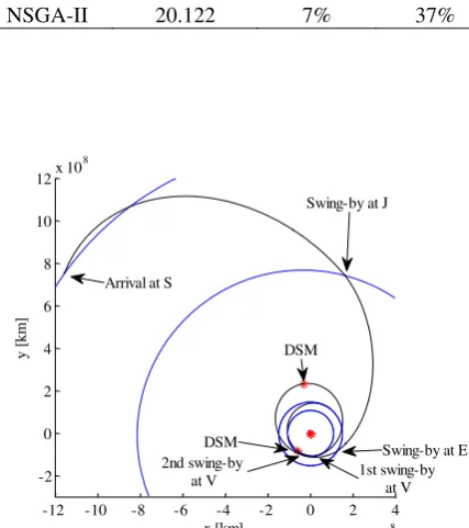
The best solution found through ACO-MGA (sequence EVVEJS) has an objective value of 6.9686 km/s: The characteristics of this solution can be found in Table 6, compared to the best solution found for the Earth-Saturn transfer problem (see http://www.esa.int/gsp/ACT/inf/op/ globopt/edvdvdedjds.htm) found with MIDACO and reproduced with the model in [3]. The trajectory of the ACO-MGA solution is shown in Fig. 9 (a), while the 3D reference solution is in Fig. 9 (b).
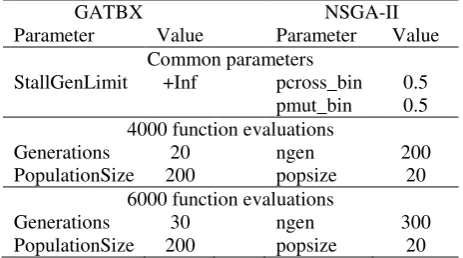
Table 5. Parameters of GATBX and NSGA-II for the Cassini test case.
GATBX NSGA-II
Parameter Value Parameter Value Common parameters
StallGenLimit +Inf pcross_bin 0.5 pmut_bin 0.5 4000 function evaluations
Generations 20 ngen 200 PopulationSize 200 popsize 20
6000 function evaluations
[image:13.612.324.556.549.678.2]It is interesting to sort the feasible sequences found by ACO-MGA according to the best objective value that they can achieve. The bar graph in Fig. 10 shows the outcome: note that every sequence has a trajectory associated to it, modelled as shown before, and thus taking into account the phasing problem. This means that these solutions could be re-optimised with a more detailed model (in particular including the third dimension), leading to actual transfer solutions. This means that ACO-MGA is a powerful tool to find feasible sequences and corresponding first-guess solutions. Launch date analysis
As mentioned before, the algorithm, at the current state, does not perform any kind of search on the launch date
0
[image:14.612.324.551.84.465.2]t . In fact, this variable is not even included in the solution vector s. Rather, if the launch date is not fixed, but a launch window is available, a systematic scan can be performed to find the best launch date, and the corresponding solutions. This procedure is not always applicable: in fact, if re-running the algorithm for a small Table 7. Comparison of the performances of ACO-MGA,
GATBX, NSGA-II over 100 runs for the Cassini problem.
Optimiser Average best value, km/s
% runs < 16 km/s
% feasible runs 4000 function evaluations
ACO-MGA 16.24 44% 91% GATBX 16.349 14% 25% NSGA-II 20.426 5% 26%
6000 function evaluations
ACO-MGA 15.434 80% 100% GATBX 16.526 17% 28% NSGA-II 20.122 7% 37%
Table 6. Characteristics of the ACO-MGA solution and the reference solutions.
Variable ACO-MGA Reference
0
v , km/s 3.14 3.259
1
v
, m/s 600 480
2
v
, m/s 350 398
3
v
, v4, v5, m/s 0 0
v, km/s 4.21 4.246
1
T, d 168 167
2
T , d 423 424
3
T , d 53 53
4
T , d 596 589
5
T , d 2290 2200
a)
-12 -10 -8 -6 -4 -2 0 2 4
x 108 -2
0 2 4 6 8 10 12x 10
8
x [km]
y [
km
]
DSM Arrival at S
Swing-by at J
Swing-by at E 1st swing-by
at V 2nd swing-by
at V DSM
b)
-12 -10 -8 -6 -4 -2 0 2 4
x 108 -2
0 2 4 6 8 10 12x 10
8
x [km]
y [
km
]
Swing-by at J
Arrival at S
2nd swing-by
at V 1st swing-byat V
Swing-by at E DSM
DSM DSM
DSM
Fig. 9: (a) ACO-MGA solution; (b) Cassini reference solution.
EVVEJS EVVEES EVEEJS EVEEES EVVVES EVVVVS
0 5 10 15 20 25
Sequence
y, km
/s
[image:14.612.58.293.102.220.2] [image:14.612.66.280.206.447.2] [image:14.612.63.289.505.657.2]change in the launch date, the solutions that ACO-MGA finds are substantially different, then the systematic scan along t0 is not feasible, and this variable must be taken into account in the optimization process. If, on the other hand, a small displacement along t0 causes a small
change in the best solution found (e.g. same planetary sequence, possibly different types of transfers, similar objective value), then the systematic scan is a tool for identifying the promising launch possibilities.
A test for verifying this assertion was run using the BepiColombo [15] transfer problem. BepiColombo is a multiple gravity assist mission to Mercury, currently under study at ESA and JAXA. In Ref. [15] an optimal transfer solution is provided, using two swing-by of Venus to reach Mercury (sequence EVVMe). The optimal launch date is found on 15 August 2013, i.e.
0 4974.5 d, MJD2000
t .
ACO-MGA was run on this transfer problem, leaving the choice of the two swing-bys among Mercury, Venus and Earth, and leaving free other transfer parameters, like the number of revolutions. The objective is to minimise the relative velocity v at Mercury.
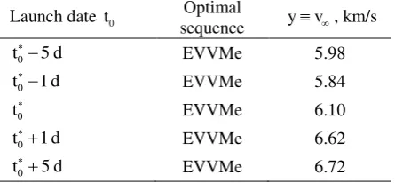
Five different launch dates, in a window of 10 days around the one chosen by ESA, were considered, and for each one of them, 100 runs were used. The corresponding best solution values are found in Table 8. The result is that the best solution is found about 1 day before t0, while earlier or later launches become less convenient. In addition, all the solutions around the ideal launch date have the same planetary sequence of swing-bys.
The discrepancy between the value of v found by ACO-MGA and the one in [15] has two causes: the first is that ACO-MGA does not take into account the inclination of the planets, and the orbit of Mercury is highly inclined. The second is that the ESA solution was found as a part of a longer trajectory, and thus with a different objective. The same reasons explain why, according to ACO-MGA, the ideal launch date is 1 day earlier. As a matter of fact, this is not a problem, and a subsequent local optimisation of the ACO-MGA solutions with a full model would tune the launch date.
[image:15.612.62.285.611.714.2]Thus, we can conclude that the systematic search can be exploited to find optimal launch dates.
Table 8: Best solutions to Mercury found by ACO-MGA for different launch dates.
Launch date t0
Optimal
sequence yv, km/s
0 5 d
t EVVMe 5.98
0 1 d
t EVVMe 5.84
0
t EVVMe 6.10
0 1 d
t EVVMe 6.62
0 5 d
t EVVMe 6.72
CONCLUSION
The paper introduced a novel formulation of the automatic complete trajectory planning problem and proposed a new algorithm (ACO-MGA), based on the ant colony paradigm, to generate optimal solutions to this problem. Each solution is a complete, unscheduled plan. Each plan is then processed through a specific model that efficiently generates families of scheduled trajectories for multi-gravity assist transfers. The 2D trajectory model proved to be accurate enough to closely reproduce known MGA transfers even with moderate inclinations. Furthermore, the scheduling of the trajectories is fast and reliable allowing for the evaluations of thousands of plans in a short time.
ACO-MGA operates an effective search in the finite space of possible plans. The algorithm demonstrated a remarkable ability to find good solutions with a very high success rate, outperforming known implementations of genetic algorithms. As ACO-MGA requires very little information on the MGA problem under investigation, it represents a valuable tool for the complete automatic design of future space missions. Future work aims at a more efficient handling of the lists, which is currently the major bottleneck of the ACO-MGA implementation.
REFERENCES
1. A. E. Petropoulos, J. M. Longuski, E. P. Bonfiglio,
“Trajectories to Jupiter via gravity assists from Venus, Earth, and Mars”, Journal of Spacecraft and Rockets, vol. 37, n. 6, p. 776-783, 2000
2. A. V. Labunsky, O. V. Papkov, K. G. Sukhanov,
“Multiple gravity assist interplanetary trajectories”,
Earth Space Institute Book Series, Gordon and Breach Science Publishers, 1998
3. M. Vasile, P. De Pascale, “Preliminary design of multiple gravity-assist trajectories”, Journal of Spacecraft and Rockets, vol. 43, n. 4, p. 794-805, 2006
4. O. Von Stryk, M. Glocker, “Decomposition of mixed-integer optimal control problems using
branch and bound and sparse direct collocation”, in
Proceedings of ADPM 2000 – The 4th International Conference on Automation of Mixed Processes: Hybrid Dynamic Systems, Dortmund, Germany, 2000
5. I. M. Ross, C. N. D'Souza, “Hybrid optimal control
framework for mission planning”, Journal of Guidance, Control, and Dynamics, vol. 28, n. 4, p. 686-697, 2005
6. B. J. Wall, B. A. Conway, “Genetic algorithms applied to the solution of hybrid optimal control
problems in astrodynamics”, Journal of Global Optimization, vol. 44, n. 4, p. 493-508, 2009
7. M. Dorigo, T. Stützle, “Ant colony optimization”, The MIT Press, Cambridge, Massachusetts, 2004 8. M. Dorigo, L. M. Gambardella, “Ant colony system:
A cooperative learning approach to the traveling
Evolutionary Computation, vol. 1, n. 1, p. 53-66, 1997
9. D. Merkle, M. Middendorf, H. Schmeck, “Ant colony optimization for resource-constrained project
scheduling”, IEEE Transactions on Evolutionary Computation, vol. 6, n. 4, p. 333-346, 2002
10. C. Blum, “Beam-ACO - Hybridizing ant colony optimization with beam search: An application to
open shop scheduling”, Computers and Operations Research, vol. 32, n. 6, p. 1565-1591, 2005
11. ESA, “Laplace mission summary”, available from:
http://sci.esa.int/science-e/www/area/index.cfm?fareaid=107, cited 9 September 2008
12. F. Peralta, S. Flanagan, “Cassini interplanetary
trajectory design”, Control Engineering Practice, vol. 3, n. 11, p. 1603-10, 1995
13. K. Deb, S. Agrawal, A. Pratap, T. Meyarivan, “A fast elitist non-dominated sorting genetic algorithm for multi-objective optimization: NSGA-II”, in
Proceedings of 6th International Conference on Parallel Problem Solving from Nature, PPSN VI, Paris, France, 2000
14. M. Vasile, E. Minisci, M. Locatelli, “On testing global optimization algorithms for space trajectory
design”, in Proceedings of AIAA/AAS Astrodynamics Specialist Conference and Exhibit, Honolulu, Hawaii, 2008
15. D. Garcia Yárnoz, P. De Pascale, R. Jehn, S.
Campagnola, C. Corral, et al., “BepiColombo
Mercury cornerstone consolidated report on mission
analysis”, ESA-ESOC Mission Analysis Office, MAO Working Paper No. 466, Darmstadt, 2006 16. M. Ceriotti, M. Vasile, C. Bombardelli, “An
incremental algorithm for fast optimisation of