Automatic MGA trajectory planning with a modified ant colony optimization algorithm

(1)

AUTOMATIC MGA TRAJECTORY PLANNING WITH A MODIFIED ANT COLONY OPTIMIZATION ALGORITHM

Matteo Ceriotti (1), Massimiliano Vasile (1) (1)

Department of Aerospace Engineering, University of Glasgow, Glasgow G12 8QQ, UK, m.ceriotti@aero.gla.ac.uk

ABSTRACT

This paper assesses the problem of designing multiple gravity assist (MGA) trajectories, including the sequence of planetary encounters. The problem is treated as planning and scheduling of events, such that the original mixed combinatorial-continuous problem is discretised and converted into a purely discrete problem with a finite number of states. We propose the use of a two-dimensional trajectory model in which pairs of celestial bodies are connected by transfer arcs containing one deep-space manoeuvre. A modified Ant Colony Optimisation (ACO) algorithm is then used to look for the optimal solutions. This approach was applied to the design of optimal transfers to Saturn and to Mercury, and a comparison against standard genetic algorithm based optimisers shows its effectiveness.

1. INTRODUCTION

In the literature on multiple gravity assist trajectories (MGA), their automatic complete design (i.e. the definition of an optimal sequence of planetary encounters and the definition of one or more locally optimal trajectories for each sequence) has been approached with several different techniques. All of them can be classified in two main categories: two level approaches and integrated approaches.

Two-level approaches split the problem into two sub-problems which are solved one after the other: firstly, a sequence (or a set of sequences) is selected, by using a simplified, low-fidelity model for representing the trajectory [1]; then, at the second level, the optimal trajectory can be searched for, within the set of selected sequences only [2], using full model. Although the number of possible planetary sequences is finite, it can be very high. Furthermore, for each sequence, there is an infinite variety of possible trajectories. The issue with two-level approaches is that if the low-fidelity model is not accurate enough, either some good sequences are discarded, or many of the retained ones can result to be actually not interesting.

As opposed to the two-level approaches, integrated approaches define a mixed integer-continuous optimization problem, which tackles both the search of the sequence and the optimization of the trajectory, using a single model, at the same time [3]. This kind of problem is known in literature as a hybrid optimization problem [4]. The main difficulty with integrated approaches is that a variation of even a single celestial body in the sequence corresponds to a substantially different set of trajectories. In addition, a variation of the length of the sequence implies varying the number of legs of the trajectory, and thus the total length of the solution vector.

The automatic design of a trajectory with discrete events was recently formulated as a hybrid optimal control problem [5], and a solution was proposed by Conway et al. [6] with a two level approach based on genetic algorithms.

(2)

optimization problems. Here the original idea behind ACO was elaborated to solve the planning problem associated to the design of MGA trajectories. In the literature, some ACO-derived meta-heuristics exist for the specific solution of different scheduling problems. In particular, Merkle et al. [8] proposed to apply ACO to the solution of the Resource-Constrained Project Scheduling Problem, while Blum, in his work [9], suggested the hybridization of Ant Colony Optimization with a probabilistic version of Beam Search for the solution of the Open Shop Scheduling problem. The paper is structured as follows: at first we will present the trajectory model and the integrated scheduling of the events; then the novel ACO-based algorithm and how the plan is constructed; finally, two case studies will demonstrate the effectiveness of the proposed approach at solving known space trajectory design problems.

2. TRAJECTORY MODEL

The trajectory model is devised having in mind the planning and scheduling process and the planning algorithm fully exploits its characteristics.

The model is based on a two dimensional linked conic approximation of the trajectory and planar orbits of the planets. The trajectory is composed of a sequence of planar conic arcs linked together through discrete, instantaneous events. In particular, the sequence is continuous in position and piecewise continuous in velocity, i.e. each event introduces a discontinuity in the velocity of the spacecraft but not in its position. The discrete events can be: launch, deep space manoeuvre (DSM), swing-by, and brake.

A final assumption of the present implementation is that all the orbits of both spacecraft and celestial bodies are direct, thus no retrograde orbits are allowed.

In summary, the proposed trajectory model is composed of: a launch from the departure celestial body; a series of deep space flight legs connected through gravity assist manoeuvres (modelled through a linked-conic approximation); an arrival at a target celestial body. Each one of these basic components will be explained in the following.

2.1 Launch

The launch event is modelled as an instantaneous change of the velocity of the spacecraft with

respect to the departure planet. The velocity change is given in terms of modulus v₀ (which depends

on the capabilities of the launcher) and in-plane direction, specified through the angle

ϕ

₀, measured counter clockwise with respect to the planet’s orbital velocity vector v_P at time of launch t₀.

0

t and

ϕ

₀ are free parameters of the model, while launch velocity modulus v₀ will be used to target the next planetary encounter and solve the phasing problem, as explained in section 2.4.

2.2 Swing-by

Gravity assist manoeuvres, or swing-bys, are modelled as instantaneous changes of the velocity vector of the spacecraft due solely to the gravity field of the planet.

Given the relative velocity vector v−_∞ before the swing-by, the physical properties of unperturbed

hyperbolic orbital motion prescribe that v_∞+ =v_∞− =v_∞, which means that the modulus of the outgoing velocity v_∞+ at infinity is known. Its direction can be computed considering the anomaly of the outgoing asymptote:

2

arccos P p

P p

r

v r

µ

θ

µ

∞

 ₋ 

= _ _

+

 

(3)

Here,

µ

_P is the gravity constant of the planet, and r_p is the radius of the pericentre of the hyperbola. The value of r_p can be used to control the magnitude of the deflection angle

(

2

)

δ

= ±

θ

∞−

π

of the incoming velocity and is limited to be above the radius of the planet, RP, to

avoid a collision, or to be above the atmosphere to avoid a re-entry. The direction of deflection is determined using a signed radius of pericentre r_ps, such that r_p = r_ps and sgn

( )

δ =sgn

( )

r_ps . Once δ is computed, the relative outgoing velocity is calculated by rotating v−_∞ in the plane of an angle δ . As for the launch velocity magnitude, the radius of pericentre r_ps is tuned to meet the terminal conditions of the transfer leg following the swing-by.

2.3 Deep space flight leg

Each deep space flight leg starts at a departure planet P_i and ends at an arrival planet P_i₊₁, and is made of two conic arcs linked, at a point M_i, through a single discrete event. The event is an instantaneous change in the heliocentric velocity vector of the spacecraft, or deep space manoeuvre, due to an ignition of the engines. In this model, we assume that the DSM is performed either at the apocentre or pericentre of the conic arc preceding the manoeuvre. In addition, the change in velocity is tangential to that arc.

For clarity, in the remainder of this section, we neglect the subscript index i of the leg in all the variables.

First arc

Let us assume that the spacecraft is at a given planet P₁ at time t₁. Its position coincides with that of the planet, which is known from the 2D ephemeris. The heliocentric velocity of the spacecraft, instead, depends on the preceding launch or swing-by event.

If the transfer leg contains a DSM, the first step is to find the position M and time t_DSM of the deep space manoeuvre. The position can either be the pericentre or the apocentre, according to a binary parameter f_{p a}_/ . The true anomaly of the DSM is θ_DSM =0 if f_{p a}_/ =0 (pericentre) or θ_DSM =π if

/ 1

p a

f = (apocentre).

The time of the DSM t_DSM is found by using the time law. The parameter n_rev_,1 is used to count the number of full revolutions before the deep space manoeuvre.

At M, the DSM is applied tangentially, being the free parameter m_DSM the magnitude and direction

of the DSM: if m_DSM is positive, the thrust is along the velocity of the spacecraft, otherwise it is against the velocity of the spacecraft. The complete state of the spacecraft at the beginning of the second arc is thus fully determined.

If the leg does not contain any DSM, i.e. m_DSM =0, the first arc is propagated up to a fictitious point

M, defined by adding an angle ∆_θ to the initial true anomaly of the spacecraft. The quantity ∆_θ is a small angular displacement, larger than the machine numerical precision, but small enough to allow for the modelling of very short transfer legs. For this work, ∆ =_θ 0.3 rad was chosen. The time t_M

at M is found by solving the time law. Parameters f_{p a}_/ and n_rev_,1 are not used.

Second arc

(4)

unfeasible, and the initial conditions of the leg, or its parameters, have to be changed. Otherwise, one of the two intersections is selected according to the binary parameter f_1/2: let us call θ_int,θ the true anomalies of the selected intersection, respectively along the orbit of the spacecraft and of the planet. From θ_int, the time t_int at which the spacecraft intersects P₂’s orbit can be computed with the time law, and considering the integer parameter n_rev_,2 counting the number of full revolutions between the point M and the orbital intersection. Fig. 1 illustrates a complete leg, including a DSM.

2.4 Solution of the Phasing Problem

In order to perform a gravity assist manoeuvre or a planetary capture, the terminal position of the spacecraft has to match that of the planet. However, at intersection time t_int, planet P2 is at true anomaly

2

P

θ , which is generally different from θ . The time of intersection is a function of the

states at the beginning of the leg, which ultimately depend on v₀ or r_ps depending on the starting event. Therefore, if we introduce the parameter λ, such that λ≡r_ps if swing-by, or λ ≡v₀ if launch.

The true anomalies of the intersection point and of the planet can be expressed as

θ λ

( )

and

( )

2

P

θ

λ

. Matching the position of the planet with that of the intersection point at time t_int (also known as the phasing problem), then, translates into finding a value λ λ= * that satisfies the equation (see Fig. 1 again):

( )

2

( )

* * *

0

P

θ λ θ λ θ λ

∆ ≡ − = (2)

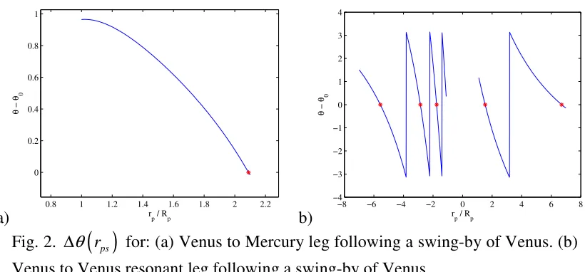
Fig. 2 (a) and (b) represent the function ∆

θ λ

( )

for different transfer cases. The case depicted in

Fig. 2 (a) shows that the function ∆

P2 is not solved, as P2 at the time of intersection is not at the intersection point.

a)

0.8 1 1.2 1.4 1.6 1.8 2 2.2

0 0.2 0.4 0.6 0.8 1 r p / Rp

θ

−

θ0

b)

−8 −6 −4 −2 0 2 4 6 8

−4 −3 −2 −1 0 1 2 3 4 r

p / Rp

θ

−

θ0

Fig. 2. ∆θ

( )

r_ps for: (a) Venus to Mercury leg following a swing-by of Venus. (b) Venus to Venus resonant leg following a swing-by of Venus.

2.5 Complete trajectory

A complete trajectory is made of a sequence of transfer legs connecting n_P +1 celestial bodies

0, ,1 nP

P P P

 

 K . The trajectory starts from P0 at time t0 with a launch event characterized by a

departure angle ϕ₀. The first leg goes from P₀ to P₁, then a number of swing-bys and interplanetary legs follow until the final planet

P

n

P . Thus, a complete trajectory with n_P +1 planets has n_P legs, and n_P −1 swing-bys.

The solution of Eq. (2) provides a complete scheduling of the trajectory given the initial time t₀ and the five parameters _DSM, _rev_,1, _rev_,2, _{p a}_/ , _1/2

i

m n n f f

 

  for every leg i=0,...,nP−1.

Since these five parameters fully characterize all possible legs from a planet P_i to a planet P_i₊₁, they are said to define a type of transfer. Conversely, because of the multiplicity of the zeros of Eq. (2), each transfer corresponds to a set of legs.

Hence, assigning a value to t₀, ϕ₀, P_i,

P

n

P , _DSM, _rev_,1, _rev_,2, _{p a}_/ , _1/2

i

m n n f f

 

  for i=0,...,nP −1 creates

a plan, or solution, which is a tree structure in which every branch, from root to leaves, is a

trajectory. Each trajectory is characterised by a different combination of v₀* and r_p* for each leg.

Swing-by or departure Selected intersection

point with planetary orbit

Destination planet at time of orbit intersection

Planetary orbits

∆θ

Transfer trajectory

nrev,1

complete revolutions Other intersection point with planetary orbit 1 P 2 P

nrev,2 complete revolutions

before interception

Tangential DSM ∆v

[image:5.595.91.501.313.504.2]

(6)

The entire tree is a complete set of trajectories from P0 to Pn_P and represents a solution of the MGA

trajectory planning problem. Thus, a plan is fully defined by assigning a value to the parameters for all i=0,...,n_P −1.

An algorithm keeps track of all the trajectories in the tree, and yields a list containing all the possible conditions of arrival at the last reachable planet. If no trajectory in the set associated to leg

i satisfies the phasing problem, then planet i+1 cannot be reached and the algorithm terminates. A partial or incomplete plan is the set of parameters sufficient to describe a solution up to leg i. Furthermore, no solution to the phasing problem exists at leg i, the plan is broken and the solution is said to be infeasible at leg i. Furthermore, an upper bound on the time of flight of the entire trajectory, or of some legs, is introduced. Trajectories that exceed the total or partial time of flight constraint are discarded from the list. The information of infeasibility at a given transfer will be used to fill in a taboo list of broken or impracticable solutions.

For each of the trajectories found, the model computes: the sum of all the deep space manoeuvres, or total ∆v and the launch excess velocity, v0; the relative velocity at the last planet, v∞; the total

time of flight of the trajectory, T.

The whole model was implemented in ANSI C and compiled as a MEX-file for interfacing with MATLAB.

3. THE ACO-MGA ALGORITHM

The model described in the previous section yields a set of scheduled trajectories provided that a complete or partial plan is available. In this section, we present an optimization procedure, based on the ant colony optimization paradigm, to explore the space of possible plans.

At first, the continuous space of the real parameters t₀, ϕ₀ and m_{DSM i} is reduced to a finite set of states. Then, the optimization algorithm, called ACO-MGA in the following, operates a search in the finite space of possible values for the design parameters. A complete description of the algorithm ACO-MGA follows.

3.1 Solution coding

In ACO-MGA, a solution is coded through a string of discrete values assigned to the parameters. However, the set of parameters discussed before is inhomogeneous, as it is made of real, integer and binary variables. In particular, t₀, ϕ₀ and m_{DSM i} are real continuous variables and need to be properly discretised. In the present implementation of ACO-MGA, the values of the departure date

0

t and the departure angle ϕ₀, are assumed to be pre-assigned and therefore the two parameters are

removed from the list of the variables. The rationale behind this choice is that, although the launch date has a great impact on the resulting trajectory, if an algorithm exists that is able to efficiently generate a complete plan for a given launch date, a systematic search can be performed along the

launch window, with a given time step. The angle ϕ₀ on the other hand can very often be estimated

depending on the mission [2].

(7)

The second element of the pair is the row index of a matrix G_i containing all possible combinations of indexes identifying the elements of the five sets: q1,i,q2,i,q3,i,q4,i,q5,i. These sets contain the

possible values for each one of the five parameters identifying the type of transfer at leg i. Thus, each row of G_i is a vector representing a different type of transfer. The parameters for the jth type of transfer for the ith leg can be obtained as follows:

( 1) ,1 ( 2) ,2 ( 3) / ( 4) 1/ 2 ( 5)

1, , ; 2, , ; 3, , ; 4, , ; 5, ,

DSM i i k rev i i k rev i i k p ai i k i i k

m =q n =q n =q f =q f =q

where k_l =G_i_,₍_{j l}_,₎,l =1,..., 5.

3.2 The taboo and feasible lists

A transfer from planet P_i to planet P_i₊₁ can be feasible or unfeasible, for the same set of parameters, depending on all the preceding legs from 1 to

(

i−1

)

. For this reason, when an infeasible leg is generated, it is necessary to store the path that led to that infeasible leg. Thus, all the parameters characterising the partial solution up to Pi+1 are stored in a taboo list.

In particular, if the problem involves nP legs, then the same number of taboo lists are used. The

taboo list of leg i contains all the partial solutions which are unfeasible at leg i (but feasible for legs 1Ki−1_{). Each taboo list is stored in a matrix, which has an arbitrary number of rows and 2}_i columns.

Dual to the list of taboo partial solutions, the feasible list stores all the solutions, which are completely feasible, i.e. reach

P

n

P . This is once more a matrix with an arbitrary number of rows and

2n_P columns.

Since each solution contained in the feasible list is complete, then it is possible to associate an objective value to each one of them. A scalar value can be computed identifying the value of the trajectories. In the following test cases, we will use, as objective value, the v_∞ and a combination of

v_∞ and T. Note that, since, in general, there is more than one trajectory for a given solution (i.e. for a given set of free design variables), the objective value of a solution is given by the best trajectory value.

3.3 Search engine

The search space is organised as an acyclic oriented tree. Each branch of the tree represents a leg of the problem, while each node (or leave) represents a different destination planet and type of transfer. A population of virtual ants are dispatched to explore the tree, searching for an optimal solution.

The search runs for a given number of iterations niter max, , or until a maximum number of objective function evaluations n_{eval max}_, has been reached. An evaluation is a call to the model, in order to compute the objective value associated to a given solution.

(8)

3.4 Solution generation

The tree is simultaneously explored, from root to leaves, by m ants. At each iteration, each one of

the m ants explores the tree independently of the others, but taking into account the information collected by all the ants at the previous iterations, through the feasible list and the taboo lists. As an ant moves along a branch, it progressively composes a complete solution. At first, each ant assigns a value to the odd entries of the solution vector, i.e. composes the sequence of planetary encounters, then it assigns a value to the even entries of the solution vector, i.e. the parameters defining the type of transfer for each legs.

Planetary sequence generation

Each ant composes a solution adding one planet at the time. As the departure planet is given, the ant has only to choose the destination planet for each leg. The choice is made probabilistically by picking from the list q_{P i}_, . The selection depends on the discrete probability distribution vector d_{P i}_,

(one for every leg) which contains the probability associated to each body in q_{P i}_, . Every time an ant is at leg i, the probability distribution vector is reset to d_{P i}_, =

[

1 1 K 1

]

T_{, i.e. all the planets have} equal probability to be chosen, and the ant sweeps the entire list q_{P i}_, substituting the identification number of each element in q_{P i}_, into the ith odd component of the partial solution vector s. Then, the feasible list is searched, for all the solutions which have a (partial) planetary sequence which matches the one in s. Say that the jth element of q_{P i}_, is added to s, and the resulting partial sequence in s matches the partial sequence of the lth solution in the feasible lists, then the probability d_{P i j}_{, ,}_{( )} associated to the jth element of q_{P i}_, is increased as follows:

( ) ( )

, , , ,

1

planet P i j P i j

l

d d w

y

← + (3)

The amount of probability which is added depends on the objective value y_l of the matching solution in the feasible list, and on the weight w_planet. Thus, the probability of choosing the jth planet increases according to how many times it generates a promising sequence (leading to a feasible solution), to the value of the feasible solution itself, and to the parameter w_planet.

This mechanism is analogous to the pheromone deposition of standard ACO and aims at driving the search of the ants toward planetary sequences, which previously led to good solutions. In fact, those planets which generate (partial) sequences that appear either frequently in the feasible list, or rarely, but with low objective function are selected with higher probability. On the other hand, the probability of selecting other planets remains positive, such that one or more ants can probabilistically choose a planet that generates an undiscovered sequence. Note that, if the feasible list is empty, then all the planets have the same probability to be selected.

The parameter w_planet controls the learning rate of the ants. A low value of w_planet will make the term w_planet y_l small, and thus the probability distribution will not change much, even if the solution appears repeatedly in the feasible list, or with low values of y. Thus, a relatively low value of w_planet will favour a global exploration of the search space, while a high value of w_planet will greatly increase the probability of choosing a planet which led to a feasible sequence. If the value of

planet

(9)

a feasible sequence, rather than trying a new one, which has not proven to be feasible. For these reasons, we can say that low values of w_planet will favour local exploration of planetary sequences. The procedure iterates for all the legs of the problem, and for all the ants. At the end, all the odd

entries of the temporary solution s contain a target planet and the planetary sequence is complete.

The next step is to find the type of transfers for each leg, thus filling the even entries of s and complete the solution.

Type of transfer generation

Once a ant has composed a temporary solution s, containing the planetary sequence, it proceeds assigning values to the even components. Similarly to the planet sequence generation, for each leg, all the available types of transfer are assigned, one at the time, to the temporary solution s. A vector

s for which a value is assigned to both the odd and even component up to leg i represents a partial

solution. Similarly to before, a vector d_{t i}_, contains the probability distribution associated to the rows of the matrix G_i. For each new partial solution, at first the taboo list is checked. If the partial solution appears in the taboo list, then it means that this solution will be unfeasible, regardless of the way the solution is completed. The probability of the type of transfer associated to that sequence is set to zero, to avoid the future selection of this type of transfer. If the partial solution does not appear in the taboo list, the feasible list is searched for any matching partial solution. For every match found, the probability distribution dt i, is modified in an analogous way as in Eq. (3). The weighing w_type is introduced, with analogous meaning to w_planet, to regulate the learning rate of the type of transfer. At the end of the solution generation step, the solution s is either discarded (infeasible) or complete. Once all the ants completed their exploration, the result is a set S of solutions (less than or equal to the number of ants m) to be evaluated.

3.5 Solution evaluation

Once a set of solutions S has been generated by the ants, each solution has to be evaluated to assess its feasibility and its objective value. This is done by calling the trajectory model.

Solutions in S are evaluated one by one, by means of the model presented before. The trajectory

model can be seen as a function which takes a solution vector s as an input, together with t₀,ϕ₀,P₀, and gives as an output either an objective value y (if the solution is feasible) or the leg l_u at which the solution becomes unfeasible. If the solution is feasible, it is stored in the feasible list and l_u =0, otherwise it is stored in the l_uth taboo list.

4. CASE STUDIES

The proposed optimisation method was applied to two case studies inspired by the BepiColombo [10] and Cassini [11] missions.

Since the launch date is not taken into account in the optimisation, in the following tests it is considered fixed. In a real mission design case, where the launch date is to be determined, the entire launch window can be discretised with a given time step, and a systematic scan of several dates

within the whole launch window should be run. The launch direction α₀ is also kept fixed in these

tests, although it is easy to find heuristics for determining the value of this parameter, or discretise it and include it in the optimisation process as an additional variable.

ACO-MGA was tested against genetic algorithms, which are known to perform well on these kinds

of problems. In particular, it was chosen to use the genetic algorithm implemented in MATLAB®

(10)

test case. While NSGA-II can deal with discrete variables, GATBX only uses real variables: a wrapper of the objective function was coded to round the continuous solution vector to the closest integer.

Due to the stochastic nature of the methods involved in the comparative tests, all the algorithms were run for 100 times. The performance index used to compare the ACO-MGA against the other global optimisers is the success rate: according to the theory developed in [13], 100 repetitions give an error in the determination for the exact success rate of less than 6%.

Some preliminary tests showed that the best performances of ACO-MGA are achieved if the algorithm is run in 2 steps, using different sets of parameters. In particular, in the first step, the weights w_planet,w_type are set to 0. Remembering Eq. (3) this choice translates into an initial pure random search. In the second step, weights are set to non-null values, to explore around the feasible solutions found.

This two-step procedure can be explained in the following way. The first step allows a random sampling of the solution space, with the aim of finding a good number of feasible solutions. This is done to prevent the algorithm to stagnate around the first feasible solution found.

The second step intensifies the search around the feasible solutions which were found at step one. Because of Eq. (3), feasible solutions with low objective value are likely to be investigated more. In addition, the random component in the process does not forbid to keep exploring the rest of the search space.

The test cases were run on an Intel® Pentium® 4 3 GHz machine running Microsoft® Windows® XP.

4.1 BepiColombo case study

In this mission, the spacecraft departs from Earth (on 15 August 2013, i.e.

0 4974.5 d, MJD2000

t = ) to reach a scientific orbit around Mercury: therefore, it is advisable to

minimise the relative velocity at arrival v_∞. The launch date has been set to match the one proposed in [10], such that a reference solution for this date is available. Three legs (and thus two swing-bys) are considered for the transfer, while the launch angle was set to ϕ₀ =π . The following set of parameters was considered:

{

}

{ }

{

}

{ }

{

}

{

}

{ }

{

}

{ }

, 1, 2, 3, 4, 5,

,3 1,3 2,3 3,3 4,3 5,3

1, 2 : Mercury, Venus, Earth ; 0 ; ; 1, 2,3, 4 ; ; 0,1

Mercury ; 50, 0, 50 m/s; 0 ; 1, 2,3, 4 ; 0,1 ; 0,1

P i i i i i i

P

i= = = = ∅ = = ∅ =

= = − = = = =

q q q q q q

Since there is no DSM in the first two legs, the parameters _rev_,1 _2,_i

i

n ∈q and _{p a}_/ _4,_i

i

f ∈q are not

influent. The number of revolutions is entirely controlled by the parameter _rev_,2 _3,_i

i

n ∈q . In general,

there is no easy way to identify whether the first or the second orbital intersection is the best one, so the binary parameter f_{1/ 2}_i was left free to be chosen by the ants. For the third leg, a DSM of 50 m/s

can be exploited to target Mercury and to reduce the v_∞ with respect to it. The departure excess velocity module v0 is constrained to be within 2 and 4 km/s, while rp for Earth, Venus and Mercury

swing-bys is between 1 and 5 R_P. The total time of flight was limited to a maximum of 10 years

(11)

All the optimisers were run for up to 2000 function evaluations. GATBX and NSGA-II were run with the settings shown in Table 1. In addition, the initial population of GATBX is spread in the whole domain.

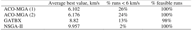
Results in the form of statistical parameters over the 100 runs are presented in Table 2. The best average value is computed on the runs which found feasible solutions only, while the value of 6 km/s as a target value for the v_∞ has been chosen to compute the success rate according to the procedure proposed in [10].

Two different set of parameters were used for ACO-MGA: (1) in Table 2 refers to a first step with 200 iterations and w_planet,w_type =0, followed by a second step of 200 iterations with

, 60 km/s

planet type

w w = ; (2) instead uses the same values for the weights, but the first step has only

60 iterations, while the second 440. This shows that a high number of iterations allocated to the second step does not necessarily improve the results, if the first step did not sample enough random points in the solution space. ACO-MGA was run on the same optimisation problem for different values of the weights, and the best results were obtained with the values mentioned before. Because of the normalisation shown in Eq. (3), the weight values appear to have general validity, and can be applied also to other transfer problems, as will be shown in the next case study.

Since the size of the population is very important for genetic-based algorithms, and it can affect the results significantly, this case study was also run 100 times with a population of 40 and 100 individuals (maintaining the predefined number of total function evaluations by varying the number of generations accordingly). For NSGA-II, it resulted that there was no noticeable change in the quality of the results over 100 runs. This is related to the fact that NSGA-II is not completely converging with 2000 function evaluations.

As a reference, by increasing the number of function evaluations to 10000, the average value of the solution from NSGA-II lowered to 7.47 km/s, with 18% below 6.5 km/s. This shows a considerable improvement but the result is still worse than ACO-MGA.

For GATBX, instead, results were changing significantly, and the settings leading to the best solutions were used.

The results in Table 2 point out that, while all the algorithms find feasible solutions in practically all the runs, the quality of the solution is much better for ACO-MGA, for either of the two different sets of settings used. Moreover, NSGA-II found a good solution only in 2 runs, and GATBX in 13. ACO-MGA, instead, found a good solution in about 25% of the runs.

[image:11.595.114.468.583.653.2]

The run time for ACO-MGA (1) was about 220 s. The simplicity of the test case, together with the implementation of ACO-MGA in a high-level language like MATLAB, makes the use of an optimisation method slower than the systematic scan of the whole solution space. Note that this will not happen in the more complex Cassini test case.

Table 1. Parameters of GATBX and NSGA-II for the BepiColombo test case.

GATBX NSGA-II

Parameter Value Parameter Value

Generations 20 ngen 100

PopulationSize 100 popsize 20

StallGenLimit +Inf pcross_bin 0.5

pmut_bin 0.5

Table 2. Comparison of the performances of ACO-MGA, GATBX, NSGA-II over 100 runs for the BepiColombo problem.

Average best value, km/s % runs < 6 km/s % feasible runs

ACO-MGA (1) 6.102 26% 100%

ACO-MGA (2) 6.176 24% 100%

GATBX 8.82 13% 98%

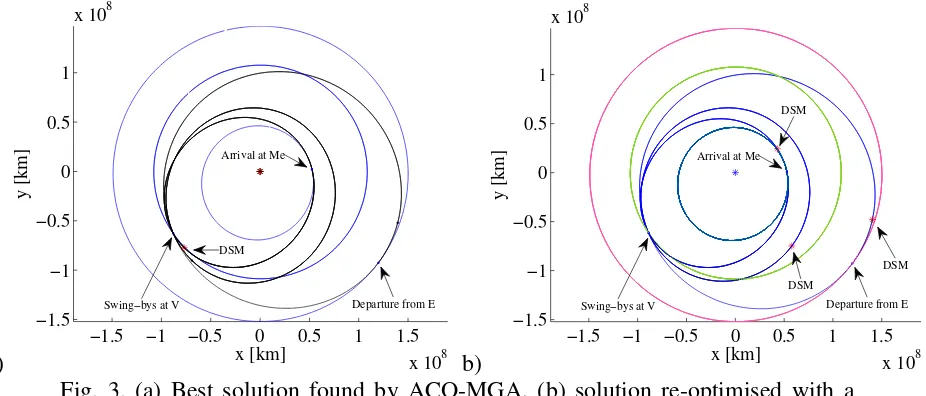
[image:11.595.108.487.694.754.2]

(12)

The best solution found by ACO-MGA is represented in Fig. 3 (a). The sequence for this solution is

EVVMe, and the objective value, i.e. the final relative velocity, is v_∞ =5.5082 km/s. The solution

exploits a 50 m/s DSM in the last leg and performs 1, 3, 4 full revolutions on each leg respectively. The validity of the model is verified by re-optimising the best solution found with ACO-MGA, but

using a full 3D model with 1 free deep space manoeuvre per leg [14], and minimising the total ∆v.

The x-y projection of the resulting trajectory is shown in Fig. 3 (b). Also, a relevant out of plane component that is introduced while considering a full 3D model with real ephemerides, and mainly due to the high inclination of Mercury.

Finally, Table 3 compares some parameters of the 2D solution with the re-optimised 3D solution and the ESOC reference solution. Note the similarity of the 3D trajectory to the one found by ESA and described in [10].

It is interesting to note that the launch velocity is higher in the 3D version mainly because of the small inclination of the planets. The v_∞ also is higher due to the inclination of the target planet but again the difference is small.

a)

−1.5 −1 −0.5 0 0.5 1 1.5

x 108

−1.5 −1 −0.5 0 0.5 1

x 108

x [km]

y [km]

Swing−bys at V Departure from E Arrival at Me

DSM

b)

−1.5 −1 −0.5 0 0.5 1 1.5

x 108

−1.5 −1 −0.5 0 0.5 1

x 108

x [km]

y [km]

DSM

Departure from E Arrival at Me

Swing−bys at V

DSM

[image:12.595.69.532.273.471.2]

Fig. 3. (a) Best solution found by ACO-MGA, (b) solution re-optimised with a full 3D model, minimising the total ∆v.

Table 3. Characteristics of the ACO-MGA solution, the re-optimised 3D solution, and the ESOC reference solution.

Variable ACO-MGA 3D optimised ESOC Variable ACO-MGA 3D optimised ESOC

0

v , km/s 3.63 3.8 3.79 v_∞, km/s 5.51 5.68 5.68

1

v

∆ , m/s 0 7 7 T₁, d 438.5 438.5 438

2

v

∆ , m/s 0 0 0 T₂, d 674.1 674 674.1

3

v

∆ , m/s 50 11 11 T₃, d 630.8 630.8 630.9

4.2 Cassini case study

Cassini is the ESA-NASA mission to Saturn. The planetary sequence designed for the mission, EVVEJS is particularly long, allowing a substantial saving of propellant. For testing the

ACO-MGA we will make use of a 5-leg trajectory, with starting date t0 = −779 d, MJD2000,

[image:12.595.298.535.530.615.2]

(13)

{

}

{ }

1, 2, 3, 4, 5,

1, 2,3 : 600, 350, 200, 0 m/s; 0 ; 0 ; 0,1 ; 0,1

4,5 : 0 ; ; 0 ; ; 0,1

i i i i i

i i

= = ± ± ± = = = =

= = = ∅ = = ∅ =

q q q q q

The planets available for swing-bys are q_{P i}_, =

{

Venus, Earth, Jupiter ,

}

i=1,.., 4, while the target planet is obviously fixed to Saturn. The number of maximum full revolutions was fixed to 0, as it can be seen from the choice of parameters n_rev_,1 and n_rev_,2. This is done to limit the total time of flight of the mission. Since the trajectory is going outwards of the orbit of the Earth, every full revolution implies more than one additional year in the transfer time. The main aim of this case study, then, is to assess the ability of finding promising planetary sequences, using deep space manoeuvres. The total number of distinct solutions for this test is 7,112,448, and the average time to evaluate a solution is 1.26 ms. This translates in 8961.7 s (or about 2.5 hours) to systematically evaluate all the solutions.

The launch excess velocity module was bounded between 2 and 4 km/s. For the swing-bys of Earth and Venus, the radii of pericentre span from 1.1 to 5 R_P. A different choice was adopted for Jupiter. In fact, the mass of this planet is considerably bigger than the masses of Venus and Earth, so higher radii of pericentre are enough to achieve considerable deviations. It was decided to consider the range 5 to 100 R_P.

Regarding the choice of the objective function, it has to be noted that for all the missions to outer planets, the time of flight becomes very important, as very long missions are needed to reach farther destinations. Even limiting the number of complete revolutions to zero, is not enough to guarantee a mission with reasonable duration. Therefore, it is important to include the total time of flight T in the objective function, in addition to the total ∆v. Since the current algorithm cannot deal with multi-objective optimisation, the total time of flight and the v_∞ are weighed inside the objective function, such that y=v_∞+σT: for this test case the weight on T was chosen to be

1 1000 km/s/d

σ

= .

The total time of flight has been limited to a maximum of 100 years: limiting the time of flight to lower values would over-constrain the search for optimal solutions. Instead, better results are obtained by allowing long solutions to be returned as feasible, and introducing their duration into the objective function.

The three optimisers were run at first for 4000 and then for 6000 function evaluations. The weights of ACO-MGA were set to w_planet,w_type =0 for the first step, and w_planet,w_type =140 km/s for the second step. With these settings, a run of ACO-MGA takes 161 s for 4000 evaluations and 273 s for 6000 evaluations. This is considerably faster than the exhaustive scan of the solution space.

The parameters used for GATBX and NSGA-II are reported in Table 4. The comparative results for the two sets of runs are shown in Table 5. It can be seen that, for 4000 evaluations, ACO-MGA found feasible solutions in 91% of the runs, compared to 25% of GATBX and 26% of NSGA-II. The average ACO-MGA solution is also slightly better than GATBX, and considerably better than NSGA-II. The performances of ACO-MGA increase significantly by using 6000 evaluations: all the runs produce a feasible solution, and in 80% of the cases, the best solution found is below 16 km/s. The average value of the solution also decreases to 15.434 km/s. It is interesting to note that, for GATBX, the average best solution found with 6000 evaluations is higher than for 4000: this is partly balanced by the fact that it finds feasible solutions in 28% of the runs. Another thing worth noticing is that NSGA-II finds more often feasible solutions than GATBX, but their quality is in average worse.

(14)

[image:14.595.106.486.111.207.2]

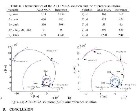
edvdvdedjds.htm) found with MIDACO and reproduced with the model in [3]. The trajectory of the ACO-MGA solution is shown in Fig. 4 (a), while the 3D reference solution is in Fig. 4 (b).

Table 4. Parameters of GATBX and NSGA-II for the Cassini test case.

Function evaluations

GATBX NSGA-II

Parameter Value Parameter Value

StallGenLimit +Inf pcross_bin 0.5

pmut_bin 0.5

4000 Generations 20 ngen 200

6000 Generations 30 ngen 300

[image:14.595.105.486.251.340.2]

Table 5. Comparison of the performances of ACO-MGA, GATBX, NSGA-II over 100 runs for the Cassini problem.

Function

evaluations Optimiser

Average best value, km/s

% runs

< 16 km/s % feasible runs

4000

ACO-MGA 16.24 44% 91%

GATBX 16.349 14% 25%

NSGA-II 20.426 5% 26%

6000

ACO-MGA 15.434 80% 100%

GATBX 16.526 17% 28%

[image:14.595.63.536.342.725.2]

NSGA-II 20.122 7% 37%

Table 6. Characteristics of the ACO-MGA solution and the reference solutions.

Variable ACO-MGA Reference Variable ACO-MGA Reference

0

v , km/s 3.14 3.259 T1, d 168 167

1

v

∆ , m/s 600 480 T2, d 423 424

2

v

∆ , m/s 350 398 T3, d 53 53

3

v

∆ , ∆v₄, ∆v₅, m/s 0 0 T4, d 596 589

v_∞, km/s 4.21 4.246 T5, d 2290 2200

a)

−10 −5 0

x 108 −2 0 2 4 6 8 10 12x 10

8

x [km]

y [km] DSM

Arrival at S

Swing−by at J

Swing−by at E 1st swing−by at V 2nd swing−by at V DSM b)

−10 −5 0

x 108

−2 0 2 4 6 8 10

12x 10

8

x [km]

y [km]

Swing−by at J

Arrival at S

2nd swing−by

at V 1st swing−by at V

Swing−by at E DSM

DSM DSM DSM

Fig. 4. (a) ACO-MGA solution; (b) Cassini reference solution.

5. CONCLUSION

(15)

processed through a specific model that efficiently generates families of scheduled trajectories for multi-gravity assist transfers. The 2D trajectory model proved to be accurate enough to closely reproduce known MGA transfers even with moderate inclinations. Furthermore, the scheduling of the trajectories is fast and reliable allowing for the evaluations of thousands of plans in a short time. ACO-MGA operates an effective search in the finite space of possible plans. The algorithm demonstrated a remarkable ability to find good solutions with a very high success rate, outperforming known implementations of genetic algorithms. As ACO-MGA requires very little information on the MGA problem under investigation, it represents a valuable tool for the complete automatic design of future space missions. Future work aims at a more efficient handling of the lists, which is currently the major bottleneck of the ACO-MGA implementation.

6. REFERENCES

[1] Labunsky A.V., Papkov O.V. and Sukhanov K.G., Multiple gravity assist interplanetary

trajectories, Earth Space Institute Book Series, Gordon and Breach Science Publishers, 1998

[2] Petropoulos A.E., Longuski J.M. and Bonfiglio E.P., “Trajectories to Jupiter via gravity assists

from Venus, Earth, and Mars”, Journal of Spacecraft and Rockets, vol. 37, n. 6, p. 776-783, 2000

[3] Vasile M. and De Pascale P., “Preliminary design of multiple gravity-assist trajectories”,

Journal of Spacecraft and Rockets, vol. 43, n. 4, p. 794-805, 2006

[4] Von Stryk O. and Glocker M., “Decomposition of mixed-integer optimal control problems using

branch and bound and sparse direct collocation”, in Proceedings of ADPM 2000 – The 4th

International Conference on Automation of Mixed Processes: Hybrid Dynamic Systems, Dortmund, Germany, 2000

[5] Ross I.M. and D'Souza C.N., “Hybrid optimal control framework for mission planning”, Journal

of Guidance, Control, and Dynamics, vol. 28, n. 4, p. 686-697, 2005

[6] Wall B.J. and Conway B.A., “Genetic algorithms applied to the solution of hybrid optimal

control problems in astrodynamics”, Journal of Global Optimization, vol. 44, n. 4, p. 493-508, 2009

[7] Dorigo M. and Stützle T., Ant colony optimization, The MIT Press, Cambridge, Massachusetts,

2004

[8] Merkle D., Middendorf M. and Schmeck H., “Ant colony optimization for resource-constrained project scheduling”, IEEE Transactions on Evolutionary Computation, vol. 6, n. 4, p. 333-346, 2002

[9] Blum C., “Beam-ACO - Hybridizing ant colony optimization with beam search: An application

to open shop scheduling”, Computers and Operations Research, vol. 32, n. 6, p. 1565-1591, 2005

[10] Garcia Yárnoz D., De Pascale P., Jehn R., et al., “BepiColombo Mercury cornerstone consolidated report on mission analysis”, ESA-ESOC Mission Analysis Office, MAO Working Paper No. 466, Darmstadt, 2006

[11] Peralta F. and Flanagan S., “Cassini interplanetary trajectory design”, Control Engineering Practice, vol. 3, n. 11, p. 1603-10, 1995

[12] Deb K., Agrawal S., Pratap A., et al., “A fast elitist non-dominated sorting genetic algorithm

for multi-objective optimization: NSGA-II”, in Proceedings of 6th International Conference on

Parallel Problem Solving from Nature, PPSN VI, Paris, France, 2000

[13] Vasile M., Minisci E. and Locatelli M., “On testing global optimization algorithms for space

trajectory design”, in Proceedings ofAIAA/AAS Astrodynamics Specialist Conference and Exhibit,

Honolulu, Hawaii, 2008