specified heat flux boundary conditions
Jianping Meng1, Yonghao Zhang1,∗, Jason M. Reese21James Weir Fluids Laboratory, Department of Mechanical & Aerospace
Engineer-ing, University of Strathclyde, Glasgow, G1 1XJ, United Kingdom
2School of Engineering, University of Edinburgh, Edinburgh, EH9 3JT, United
King-dom
Abstract. We investigate unidirectional rarefied flows confined between two infinite parallel plates with specified heat flux boundary conditions. Both Couette and force-driven flows are considered. The flow behaviors are analyzed numerically by solv-ing the Shakhov model of the Boltzmann equation. We find that the existence of an zero heat flux wall can significantly influence the flow behavior, including the velocity slip and temperature jump at the wall, especially for high-speed flows. The predicted bimodal-like temperature profile for force-driven flows cannot even be qualitatively captured by the Navier-Stokes-Fourier equations.
AMS subject classifications: 76P05, 82B40
Key words: specified heat flux boundary, rarefied gas flow, S model, discrete velocity method
1
Introduction
In a broad range of engineering applications, the characteristic spatial scale is compara-ble to the mean free path of the working gas. These application range from high altitude and high speed space vehicles [1] to Micro-Electro-Mechanical systems (MEMS) [2]. In such conditions, typically, the conventional Navier-Stokes-Fourier (NSF) equations are invalid as rarefaction effects become substantial. Kinetic methods such as direct simu-lation Mote Carlo (DSMC) [3] or direct solution of the Boltzmann equation [4] become neccessary. However, the computational costs of these methods are high. In particular, the signal/noise ratio is typically low for flows in MEMS making the computational cost significant for DSMC. Various techniques have been proposed to improve computational efficiency, e.g. [5–8].
Thermal management is often of great importance in many applications, e.g., re-entry vehicle thermal protection systems in which insulation techniques are used. To
∗Corresponding author. Email address: [email protected] (J. P. Meng),
[email protected](Y. H. Zhang),[email protected](J. M. Reese)
describe such systems, it is important to employ heat flux boundary conditions so that the heat exchange between the system and the surroundings can be controlled [9–18]. Particularly, in a well insulated surface, the adiabatic boundary condition may be-come appropriate for flow modeling. For this purpose, a immediate way is to set the accommodation coefficient in the commonly used Maxwell-type boundary to zero, i.e., full specular reflection, see the discussion in [11] and an example in [15]. Naturally, this kind of implementation is typically corresponding to a smooth surface. How-ever, for rough surfaces, the heat exchange control is also possible. Therefore, it is necessary to discuss the specified heat flux boundary condition under a full diffuse-reflection condition. A few implementations have been explicitly discussed for the DSMC method [9, 10]. However, in terms of kinetic model equations, there is lack of such discussion and understanding of flow features even for simple flows.
In this paper, we report numerical investigations of rarefied gas flows confined be-tween two parallel infinite plates. We solve the Shakhov model (S model) of the Boltz-mann equation [19, 20]. While one plate is set to be with specified heat flux (mainly zero flux), the other one has a fixed temperature. Here we suppose that the zero heat
flux boundary can closely resemble the adiabatic boundary condition†. The
numeri-cal method we use is based on the deterministic discrete velocity method (see [21] and reference therein). Both a Couette flow and a force-driven Poiseuille flow are examined.
2
Formulation of problems
2.1 Specification
The monatomic gas is confined between two parallel infinite plates located at y=0 and y=L. The top plate (y=L) has a fixed temperature,T0, and the bottom one (y=0) hasa
zero heat flux. In the Couette flow, the two plates move oppositely with the same speed
Uw. For the Poiseuille flow, the gas is subject to a uniform external force in thexdirection, i.e. in the direction parallel to the plates.
2.2 Model
In order to capture rarefaction effects, we solve the S model of the Boltzmann equation which is given as:
∂f ∂t +c·
∂f ∂r+g·
∂f ∂c=
1
τ(fS−f),
where f(r,c,t)is the single molecular velocity distribution function, which describes the number (or portion) of molecules in the volumedrcentered at the positionr=(x,y,z)with velocities withindcaround the velocityc= (cx,cy,cz)at timet. Based on this distribution
†Under rarefied conditions, it becomes rather difficult to precisely define the adiabatic boundary condition,
function, macroscopic quantities such as gas densityρ, velocityu, temperatureT, stress tensorPand heat fluxqcan be obtained from its moments i.e.,
ρ[1,ui,3RT,Pij,2qi] =
Z
[1,ci,CiCi,CiCj,CiCjCj]f dc,
where C=c−u is the peculiar molecular velocity and R is the gas constant. τ is the relaxation time with the form ofτ=p/µwherepis the pressure andµthe viscosity. The body force g= (gx,gy,gz)is assumed to be independent of the molecular velocity. The “equilibrium” function fSis proposed to be
fS=feq
1+1−Pr
5
2qiCi pRT C2 2RT− 5 2 , (2.1)
where feqis the Maxwellian distribution
feq=ρ 1 2πRT 3/2 exp − C 2 2RT . (2.2)
and Pr is the Prandtl number.
It is convenient to introduce the following dimensionless quantities,
ˆ xk=
xk
L, uˆk= uk √
RT0
, tˆ=
√ RT0t
L , gˆk= Lgk RT0
, cˆk= ck √
RT0
, Tˆ= T
T0
,
ˆ
f= f(RT0) 3/2
ρ0
, ρˆ= ρ ρ0
, pˆ= p
p0
, µˆ= µ µ0
, qˆi= qi p0
√ RT0
, Pˆij= Pij p0
.
Here, we use the subscript 0 to denote the reference quantities. For the present problems, most of them are corresponding to quantities at the top plate, except that the densityρ0
should be understood as the average density. With these non-dimensional quantities, the governing equation can then be rewritten as
∂fˆ ∂tˆ
+cˆk ∂fˆ ∂xˆk
+gˆk ∂fˆ ∂cˆk
=− p0L µ0 √ RT0 ˆ p ˆ µ( ˆ
f−fˆeq) =−ρˆTˆ
(1−ω)
K (fˆ−fˆ
S), (2.3)
whereKis defined as
K=µ0
√ RT0
p0L
.
The relevant macroscopic quantities become
ˆ ρ ˆ ρuˆi
ˆ Pij 3 ˆρTˆ
2 ˆqi = Z ˆ f 1 ˆ ci ˆ CiCˆj
ˆ CiCˆi ˆ CiCˆjCˆj
The temperature-dependent viscosity can be expressed as µ/µ0= (T/T0)ω, whereω is related to the molecular interaction model, varing from 0.5 for hard-sphere molecular interactions to 1 for Maxwell molecules. The hat symbol will be omitted hereafter for clarity. A rescaled Knudsen number,
Kn=
r π
2K,
is used throughout this work.
3
Numerical method
3.1 Equations of marginal distribution functions
As the flows considered here are one-dimensional, we can introduce the following marginal velocity distribution functions, and the corresponding parts for the “equilibrium” distri-bution: ϕa ϕb ϕc ϕd ϕe ϕf = Z ∞ −∞ Z ∞ −∞ 1 cx c2x c2z c3
x cxc2z
f dcxdcz, (3.1)
ϕas ϕbs ϕcs ϕds ϕes ϕf s
=R∞ −∞R−∞∞
1 cx c2x c2z c3
x cxc2z
fSdcxdcz=ρe
−c
2 y 2T √
2πT×
1− 1
5ρT3cyqy(Pr−1)(c
2
y−3T)
1
5ρT3(Pr−1)(−c
3
yqyux−c2yqxT+3cyqyTux+qxT2)+ux
1
5ρT3(Pr−1)(−c
3
yqy(T+u2x)−2c2yqxTux+cyqyT T+3u2x
+2qxT2ux)+T+u2x
1
5ρT2cy(Pr−1)qy(T−c
2
y)+T −1
5ρT3(Pr−1)(c
3
yqyux(3T+u2x)+3cy2qxT(T+u2x)−3cyqyTux(T+u2x)+3qxT2(T−u2x))+ux(3T+u2x) Tux−5ρ1T2(Pr−1)(qxT(c2y+T)+cyqyux(c2y−T))
With these marginal distribution functions, the macroscopic quantities in Eq. (2.4) can be calculated as ρ ρux 3ρT Pxx Pxy Pyy Pzz 2qx 2qy = Z ∞ −∞ ϕa ϕb ϕc+ϕd+c2yϕa
ϕc ϕbcy c2
yϕa ϕd
−3uxϕc+ϕe−uxc2yϕa+c2yϕb−uxϕd+ϕf cy(−2uxϕb+ϕc+c2yϕa+ϕd)
dcy+ 0 0 −ρu2
x −ρu2x
0 0 0 2ρu3x
0 .
It is worth noting that, for the unidirectional flows considered here, there are some addi-tional relations, i.e.uy=uz=0,Pxz=Pyzandqz=0 [23]. Now let
φ= ϕa ϕb ϕc ϕd ϕe ϕf
, φe= ϕas ϕbs ϕcs ϕds ϕes ϕf s
, S=gx 0 ϕa 2ϕb 0 3ϕc ϕd ,
then the governing equation for the six distribution functions can be written as
∂φ ∂t +cy
∂φ ∂y=
1 KρT
(1−ω)(
φe−φ)+S. (3.3)
In particular, if the problem is steady, Eq. (3.3) can be further reduced to
cy ∂φ ∂y=
1 KρT
(1−ω)(
φe−φ)+S, (3.4)
where the time variable is eliminated. In these equations, the corresponding differential force terms have been transformed into the non-differential source term S by utilizing integration by parts, see [24] for details.
3.2 Scheme
more points near the boundaries. To construct this kind of grids, we first obtain a distri-bution of grid points that become highly dense near the middle point of the channel by using
yi=αsinh "
sinh−1 21α
(2i−N)
N
#
+1
2, i=0...N, (3.5)
where N is the total number of grid points and α is the parameter determining the nonuniformity. The grid system can then be made instead denser near the wall by utiliz-ing symmetry and translation relations.
Regarding the numerical scheme, we employ a second-order upwind scheme except in the near-wall region where a first-order upwind scheme is used. Therefore, the evolu-tion ofφcan be written associated
φi=
cy ηi2φi−1−φi−2
+dyiηi(ηi−1)(wiφe,i+Si)
(ηi−1)(ηicy+cy+dyiηiwi)
, cy>0, i=2...N (3.6)
and
φ1=
cyφ0+dy1S1+dy1w1φe,1
cy+dyw1
, cy>0, (3.7)
where
wi=
ρiTi1−ω
K , (3.8)
dyi=yi−yi−1, i=1...N,
and
ηi=
dyi+dyi−1
dyi
, i=2...N.
For simplicity, the rules forcy<0 are omitted here; they can be easily obtained in a manner similar to the above.On the other hand, convergence tests show that the whole scheme can actually achieve a second-order accuracy even at the wall point although a first order scheme is used. This can be attributed to the usage of non-uniform grid. The accuracy near wall is effectively improved by the very small grid size.
3.3 Boundary condition
In the present simulations, diffuse reflection boundary conditions are employed. The top plate has a fixed temperature while the bottom platehas a specified heat flux. For convenience, the implementation details of both fixed-temperature and specified heat
flux boundarywill be discussed using the bottom wall as an example, which can then be
straightforwardly applied to the top plate as required.
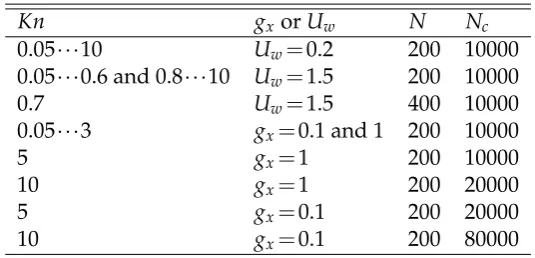
Kn gxorUw N Nc 0.05···10 Uw=0.2 200 10000 0.05···0.6 and 0.8···10 Uw=1.5 200 10000
0.7 Uw=1.5 400 10000
0.05···3 gx=0.1 and 1 200 10000
5 gx=1 200 10000
10 gx=1 200 20000
5 gx=0.1 200 20000
[image:7.595.173.441.107.236.2]10 gx=0.1 200 80000
Table 1: Discretization systems for the simulated cases
written as follows,
f(y=0,cy>0) = ρw
(2πTw)3/2 exp
− Cw2
2Tw
, (3.9)
where Cw is the peculiar molecular velocity at the wall, i.e. c−uw. To implement the specific fixed-temperature andspecified heat flux boundary conditons, we need to de-termine the corresponding macroscopic properties according to the related conservation laws. For simplicity, we first write down the incoming mass flux and heat flux as
Min=
Z
cy<0
cyf(y=0,cy<0)
dc, (3.10)
Hin=1
2 Z
cy<0
cyC2wf(y=0,cy<0)
dc. (3.11)
According to the princile of dissfuse reflection boundary conditons, the outgoing mass
flux and heat flux can be easiy calcualted ifρw andTwis first supposed to be known,
i.e.,
Mout= Z
cy>0
cy ρw
(2πTw)3/2 exp
−C
2
w
2Tw
dc=ρw
√ Tw √
2π
, (3.12)
and
Hin=1
2 Z
cy<0
cyC
2
w ρw
(2πTw)3/2 exp
− C
2
w
2Tw
d
c=2
r 2 πρwT
3/2
w . (3.13)
If the wall temperature is fixed, we can use the mass conservation law to determine density, i.e. the incoming mass flux is equal to the outgoing mass flux. Through straightforward calculations, the density at wall is given as
ρw= r
2π
Tw
For the wall with specified heat flux, we need to determine both density and tem-perature via mass conservation and the specified heat flux, i.e., we need to solve two equations as follows,
Mout−Min=0 (3.15)
and
Hout−Hout=qyw, (3.16)
where qyw denotes the specified heat flux at wall. By solving the two equations, the
density and temperature can be written as
ρw=
2√2πM3/2
in p
Hin+qyw
(3.17)
and
Tw=
Hin+qyw
4Min . (3.18)
Specifically, ifqywis set to be zero, the density and the temperature are
ρw=
2√2πM3/2in
√
Hin (3.19)
and
Tw= Hin
4Min, (3.20)
Here, we will mainly study the effect of zero heat flux boundary condition and we suppose that the this boundary condition can closely resemble the adiabatic boundary
condition. For the marginal distribution functions, the boundary Eq. (3.9) condition can
be transformed to
ϕaw ϕbw ϕcw ϕdw ϕew ϕf w
=
Z ∞
−∞ Z ∞
−∞
1 cx c2x c2
z c3x cxc2z
feq,wdcxdcz=
ρwexp(− c2
y
2Tw)
√ 2πTw
1 uw Tw+u2w
Tw
(3Tw+u2w)uw Twuw
.
4
Numerical results
0 0 . 2 0 . 4 0 . 6 0 . 8 1 - 0 . 2
- 0 . 1
0
0 . 1 0 . 2
K n = 0 . 1 K n = 0 . 5 K n = 1 K n = 5
ux
Y 0 0 . 2 0 . 4 0 . 6 0 . 8 1
0
1 . 0 0 1 . 0 1 1 . 0 2 1 . 0 3
K n = 0 . 1 K n = 0 . 5 K n = 1 K n = 5
T
Y
0 0 . 2 0 . 4 0 . 6 0 . 8 1
0
1 . 0 0 1 . 0 1 1 . 0 2 1 . 0 3 1 . 0 4 1 . 0 5
K n = 0 . 1 K n = 0 . 5 K n = 1 K n = 5 P x x
Y 0 0 . 2 0 . 4 0 . 6 0 . 8 1
- 0 . 1 5 - 0 . 1 2 - 0 . 0 9 - 0 . 0 6 - 0 . 0 3
0
K n = 0 . 1 K n = 0 . 5 K n = 1 K n = 5
P x y
Y
0 0 . 2 0 . 4 0 . 6 0 . 8 1
- 0 . 0 2 - 0 . 0 1
0
0 . 0 1 0 . 0 2
K n = 0 . 1 K n = 0 . 5 K n = 1 K n = 5
q x
Y 0 0 . 2 0 . 4 0 . 6 0 . 8 1
0
0 . 0 0 8 0 . 0 1 6
0 . 0 2 4 K n = 0 . 1
K n = 0 . 5 K n = 1 K n = 5
q y
[image:9.595.107.512.154.600.2]Y
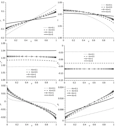
Figure 1: Profiles of macroscopic quantities for Couette flows with Uw=0.2. Adiabatic boundary at Y=0,
0 0 . 2 0 . 4 0 . 6 0 . 8 1 - 1 . 5
- 0 . 7 5
0
0 . 7 5 1 . 5
K n = 0 . 1 K n = 0 . 5 K n = 1 K n = 5
u x
Y 0 0 . 2 0 . 4 0 . 6 0 . 8 1
0
1 . 0 1 . 5 2 . 0 2 . 5
K n = 0 . 1 K n = 0 . 5 K n = 1 K n = 5
T
Y
0 0 . 2 0 . 4 0 . 6 0 . 8 1
0
2 . 0 2 . 4 2 . 8 3 . 2
K n = 0 . 1 K n = 0 . 5 K n = 1 K n = 5
P x x
Y 0 0 . 2 0 . 4 0 . 6 0 . 8 1
- 1 . 5 - 1 . 0 - 0 . 5
0
K n = 0 . 1 K n = 0 . 5
K n = 1 K n = 5
P x y
Y
0 0 . 2 0 . 4 0 . 6 0 . 8 1
- 2 . 4 - 1 . 8 - 1 . 2 - 0 . 6
0
0 . 6
K n = 0 . 1 K n = 0 . 5 K n = 1 K n = 5 q x
Y 0 0 . 2 0 . 4 0 . 6 0 . 8 1
0
0 . 6 1 . 2 1 . 8
K n = 0 . 1 K n = 0 . 5 K n = 1 K n = 5
q y
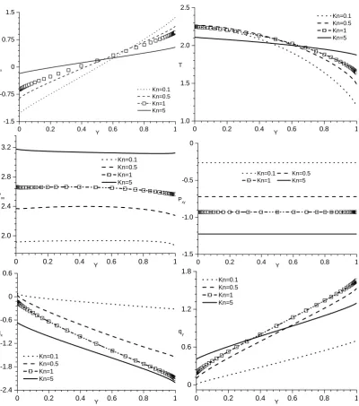
[image:10.595.81.482.150.604.2]Y
Figure 2: Profiles of macroscopic quantities for Couette flows with Uw=1.5. Adiabatic boundary at Y=0,
0 . 1 1 1 0
0
0 . 1 0 . 2 0 . 3 0 . 4
0 . 5 B o t t o m U
w= 1 . 5 T o p U w= 1 . 5 B o t t o m U
w= 0 . 2 T o p U w= 0 . 2
V
e
lo
c
it
y
s
lip
K n 0 . 1 1 1 0
0
0 . 0 4 0 . 0 8
0 . 1 2 U w= 1 . 5
U w= 0 . 2
T
e
m
p
e
ra
tu
re
j
u
m
p
[image:11.595.108.512.108.256.2]K n
Figure 3: Velocity slip at the bottom (zero heat flux) and top (fixed-temperature) plates and temperature jump at the top plate, for Couette flows. The velocity slip is re-normalized by the velocity difference of the two moving plates, and the temperature jump is re-normalized by the square of the velocity difference.
Both types of error are evaluated at the points [0,0.1,0.2,···,1] including the boundary points. If both types of errors for the temperature and velocity in the coarser system are less than 1% in comparison with the finer system, the coarser system is regarded as appropriate. According to these criteria, we determine an appropriately discretized system foreachsimulated case, which are listed in Table 1. In terms of the truncation of molecular velocity space, we choose the range[−20,20], which produces nearly identical results for the force-driven flow withKn=0.05 andgx=1 with the range[−30,30].
Typical results for Couette flows are presented in Figs. 1 – 3. In Figs. 1 and 2 it is found that the viscous heating effect can induce a larger temperature rise at the bottom
wall. For bothUw=0.2andUw=1.5the temperature keeps rising at the top wall with
the increasing Knudsen number in the presented region. However, at the bottom wall, it first increases then decreases. For the velocity, same trends are kept for both walls.
In Fig. 3, it is seen that the effect of the zero heat flux boundary on the velocity profile is significant for the high-speed case as we can observe significantly different velocity slips at the bottom and top plates. Specifically, the velocity slip at the bottom (zero heat flux) plate is larger. Interestingly, for the low-speed case, the effect on ve-locity slip is small. At the top plate, we observe that the temperature jump effect is relatively stronger for the lower speed case, in comparison to the higher speed case.
Regarding the heat flux, it is of interest to observe that there can be non-zero
span-wise heat fluxqyat the bottom wall for the larger Knudsen numbers, although a zero
heat flux is prescribed. This is certainly due to the non-continuum effect and may be understood as a kind of heat flux jump. For the stream-wise component, we ale observe non-zero values which can not be captured by the NSF equations.
For the shear stressPxxandPxy, they show similar behaviors for both of the
higher-speed and lower-higher-speed cases. Again, the trace-free part of shear stressPxx−Tis
appar-ently not zero, which can be be captured by the NSF equations.
0 0 . 2 0 . 4 0 . 6 0 . 8 1
0
0 . 1 0 . 2 0 . 3
K n = 0 . 1 K n = 0 . 5 K n = 1 K n = 5 u x
Y 0 0 . 2 0 . 4 0 . 6 0 . 8 1
1
0
1 . 0 1 1 . 0 2 1 . 0 3 1 . 0 4
K n = 0 . 1 K n = 0 . 5 K n = 1 K n = 5
T
Y
0 0 . 0 0 . 2 0 . 4 0 . 6 0 . 8 1 . 0 1
1
1 . 0 1 1 . 0 2 1 . 0 3 1 . 0 4 1 . 0 5
K n = 0 . 1 K n = 0 . 5 K n = 1 K n = 5
P
x x
Y 0 0 . 2 0 . 4 0 . 6 0 . 8 1
- 0 . 0 6 - 0 . 0 3
0
0 . 0 3 0 . 0 6
K n = 0 . 1 K n = 0 . 5 K n = 1 K n = 5
P
x y
Y
0 0 . 2 0 . 4 0 . 6 0 . 8 1
- 0 . 0 5 - 0 . 0 4 - 0 . 0 3 - 0 . 0 2 - 0 . 0 1
0
0 . 0 1 0 . 0 2
K n = 0 . 1 K n = 0 . 5 K n = 1 K n = 5
q
x
Y 0 0 . 2 0 . 4 0 . 6 0 . 8 1 . 0
0
0 . 0 0 5 0 . 0 1 0 . 0 1 5
K n = 0 . 1 K n = 0 . 5 K n = 1 K n = 5
q y
[image:12.595.80.485.157.603.2]Y
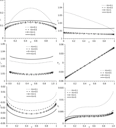
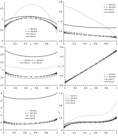
Figure 4: Profiles of macroscopic quantities for force-driven Poiseuille type flows with gx=0.1. Adiabatic
0 0.2 0.4 0.6 0.8 1 0
2 4 6 8
NSF S model
T
em
pe
ra
tu
re
Y
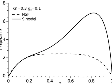
[image:13.595.209.405.107.254.2]Kn=0.3 gx=0.1
Figure 5: Comparison of temperature profiles predicted by the S model and the NSF equation atKn=0.3and gx=0.1. The temperature profiles as shown are deducted by data belonging to lines connecting points at the
top and bottom plates and then enlarged by10000times respectively. The velocity slip boundary condition is used for both two walls. Whie the temperature jump boundary condition is used at the top wall and the zero heat flux (temperature gradient) boundary condition is used at the bottom wall.
Couette flow cases, the zero heat flux boundaryinduces significantly different velocity slips at the bottom and top plates for the case ofgx=1. Different from the Couette flow, the velocity slip at the bottom wall becomes smaller as the external force increases. Again there is nearly no difference in velocity slip at the two walls for the small force cases and the temperature jump effect is relatively stronger than the the large force case.
It is interesting to note that, similar to the case of two fixed-temperature plates, we can find that the temperature profiles are qualitatively different from the NSF prediction for a range of Knudsen numbers. For instance, as shown in Fig. 5, we can see bimodal-like temperature distribution although the two tops are unsymmetrical here. This is qualita-tively different from the NSF prediction. Again the temperature near the zero heat flux wall is always the highest.
Similar to the Couette flow, heat flux jump is observed at the bottom wall. Also, there are non-zero stream-wise heat flux component and non zero trace-free shear
stressPxx−T.
In Fig. 8, we can see that, similar to cases with fixed temperature boundary at two
walls, the Knudsen minimum in the mass flow rate occurs at aroundKn=1. Since the
viscous heating effect consumes more input work in the larger force case, the mass flow rates are generally larger for the smaller force case.
5
Concluding remarks
macro-0 0 . 2 0 . 4 0 . 6 0 . 8 1
0
0 . 5
1
1 . 5
K n = 0 . 1 K n = 0 . 5 K n = 1 K n = 5 u x
Y 0 0 . 2 0 . 4 0 . 6 0 . 8 1
1 . 2 1 . 6
2
2 . 4 2 . 8
K n = 0 . 1 K n = 0 . 5 K n = 1 K n = 5
T
Y
0 0 . 2 0 . 4 0 . 6 0 . 8 1
1 . 2 1 . 6
2
2 . 4 2 . 8 3 . 2
K n = 0 . 1 K n = 0 . 5 K n = 1 K n = 5
P x x
Y 0 0 . 2 0 . 4 0 . 6 0 . 8 1
- 0 . 6 - 0 . 3
0
0 . 3 0 . 6
K n = 0 . 1 K n = 0 . 5 K n = 1 K n = 5 P x y
Y
0 0 . 2 0 . 4 0 . 6 0 . 8 1
- 1
0
1
2
3
4
K n = 0 . 1 K n = 0 . 5 K n = 1 K n = 5 q x
Y 0 0 . 2 0 . 4 0 . 6 0 . 8 1
0
0 . 4 0 . 8 1 . 2
K n = 0 . 1 K n = 0 . 5 K n = 1 K n = 5
q
y
[image:14.595.82.484.147.611.2]Y
Figure 6: Profiles of macroscopic quantities for force-driven Poiseuille type flows withgx=1. Adiabatic boundary
0.1 1 10 0
0.4 0.8
1.2 Bottomgx=1
Top gx=1
Bottomgx=0.1
Top gx=0.1
V
el
oc
ity
sl
ip
Kn 0.1 1 10
0 0.4 0.8 1.2 1.6 2 2.4 2.8
gx=1
gx=0.1
T
em
pe
ra
tu
re
ju
m
p
[image:15.595.107.511.104.258.2]Kn
Figure 7: Velocity slip at the bottom (zero heat flux)and top (fixed-temperature) plates and temperature jump at the top plate, for force-driven Poiseuille type flows. The velocity slip is re-normalized by the force magnitude, and the temperature jump is re-normalized by the square of the force magnitude.
0.1 1 10
0 0.8 1.6 2.4 3.2
gx=1
gx=0.1
M
as
s
flo
w
ra
te
Kn 0.1 1 10
0 5 10
gx=1
gx=0.1
H
ea
tf
lo
w
ra
te
Kn
Figure 8: Mass and heat flow rate for force-driven Poiseuille type flows of different Kn. Both fluid quantities are re-normalized by the force magnitude.
scopic fluid quantities can become unsymmetrical. Specifically, the temperature rise at the zero heat flux wall are higher than that at the fixed-temperature plate. When the
viscous heating effect is strong (e.g. Uw=1.5, or gx=1), the velocity slips at the two
[image:15.595.107.512.334.484.2]Acknowledgments
This work was financially supported by the Engineering and Physical Sciences Research Council of the UK under Grant Nos. EP/I036117/1 and EP/I011927/1. Yonghao Zhang would also like to thank the Royal Academy of Engineering and the Leverhulme Trust for the award of a RAEng/Leverhulme Senior Research Fellowship.
References
[1] M. S. Ivanov and S. F. Gimelshein. Computational hypersonic rarefied flows. Annu. Rev.
Fluid Mech., 30(1) (1998), 469–505.
[2] Chih-Ming Ho and Yu-Chong Tai. Micro-electro-mechanical-systems (MEMS) and fluid flows.Annu. Rev. Fluid Mech., 30(1) (1998), 579–612.
[3] G. A. Bird. Monte Carlo simulation of gas flows.Annu. Rev. Fluid Mech., 10(1) (1978), 11–31. [4] S. M. Yen. Numerical solution of the nonlinear Boltzmann equation for nonequilibrium gas
flow problems. Annu. Rev. Fluid Mech., 16(1) (1984), 67–97.
[5] Gregg A. Radtke, Nicolas G. Hadjiconstantinou, and Wolfgang Wagner. Low-noise Monte Carlo simulation of the variable hard sphere gas. Phys. Fluids, 23(3) (2011), 030606.
[6] H. Struchtrup. Derivation of 13 moment equations for rarefied gas flow to second order accuracy for arbitrary interaction potentials.Multiscale Model.Simul., 3(1) (2005), 221–243. [7] Xiaojun Gu and David R. Emerson. A high-order moment approach for capturing
non-equilibrium phenomena in the transition regime. J. Fluid Mech., 636(-1) (2009), 177–216. [8] Jianping Meng, Yonghao Zhang, Nicolas G. Hadjiconstantinou, Gregg A. Radtke, and
Xi-aowen Shan. Lattice ellipsoidal statistical BGK model for thermal non-equilibrium flows. J.
Fluid Mech., 718 (2013), 347–370.
[9] H. Akhlaghi, E. Roohi and S. Stefanov, A new iterative wall heat flux specifying technique in DSMC for heating/cooling simulations of MEMS/NEMS, Int. J. Therm. Sci., 59 (2012), 111-125.
[10] Q. W. Wang, C. L. Zhao, M. Zheng and N. Y. E. Wu, Numerical investigation of rarefied diatomic gas flow and heat transfer in microchannel using dsmc with heat flux specified boundary conditiond part I: Numerical method and validation,Numerical Heat Transfer Part B, 53 (2008), 160-173.
[11] T. Klinc and I. Kuˇser Slip coefficients for general gas-surface interaction, Phys. Fluids, 15 (1972), 1018–1022
[12] A. A. Alexeenko, D.A. Levin, S. F. Gimelshein, R. J. Collins and G.N.Markelov. Numerical simulation of high-temperature Gas flows in a millimeter-Scale thruster , J. Therm. Heat
Trans., 16 (2002), 10–16.
[13] G. N. Markelov, A. N. Kudryavtsev and M. S. Ivanov, Rarefaction effects on separation of hypersonic laminar flows,AIP Conference Proceedings, 585 (2001), 707.
[14] G. N. Markelov and M. S. Ivanov, Numerical study of 2D/3D micronozzle flows, AIP
Conference Proceedings, 585 (2001), 539.
[15] N Sengil and F. O. Edis. Implementation of parallel DSMC method to adiabatic piston prob-lem. InParallel Computational Fluid Dynamics 2007, volume 67 ofLecture Notes in
[16] Alireza Mohammadzadeh, Ehsan Roohi, Hamid Niazmand, and Stefan Stefanov. Dsmc solution for the adiabatic and isothermal micro/nano lid-driven cavity. InProceedings of the
3rd GASMEMS Workshop - Bertinoro, 2011.
[17] Rakesh Kumar, Evgeny Titov, and Deborah Levin. Comparison of statistical BGK and DSMC methods with theoretical solutions for two classical fluid flow problems. InFluid Dynamics
and Co-located Conferences, American Institute of Aeronautics and Astronautics, 2009.
[18] Jonathan M. Burt and Iain D. Boyd. Evaluation of a particle method for the ellipsoidal statis-tical Bhatnagar-Gross-Krook equation. In44thAIAA Aerospace Sciences Meeting and Exhibit, 2006.
[19] E. M. Shakhov. Generalization of the Krook kinetic relaxation equation. Fluid Dyn., 3(5) (1968), 95–96.
[20] E. M. Shakhov. Approximate kinetic equations in rarefied gas theory. Fluid Dyn, 3(1) (1968), 112–115.
[21] Tadeusz Platkowski and Reinhard Illner. Discrete velocity models of the Boltzmann equa-tion: A survey on the mathematical aspects of the theory.SIAM Review, 30(2) (1988), 213–255. [22] Yoshio Sone, Kinetic theory and fluid Dynamics, BIRKH ¨AUSER2002.
[23] Kazuo Aoki, Shigeru Takata, and Toshiyuki Nakanishi. Poiseuille-type flow of a rarefied gas between two parallel plates driven by a uniform external force. Phys. Rev. E, 65 (2002), 026315.