parameters: Some case studies
Nguyen Dang and Patrick De Causmaecker
Department of Computer Science, CODeS & imec-ITEC KU Leuven, Belgium
Abstract. Modern high-performing algorithms are usually highly pa-rameterised, and can be configured either manually or by an automatic algorithm configurator. The algorithm performance dataset obtained af-ter the configuration step can be used to gain insights into how different algorithm parameters influence algorithm performance. This can be done by a number of analysis methods that exploit the idea of learning pre-diction models from an algorithm performance dataset and then using them for the data analysis on the importance of variables. In this pa-per, we demonstrate the complementary usage of three methods along this line, namely forward selection, fANOVA and ablation analysis with surrogates on three case studies, each of which represents some special situations that the analyses can fall into. By these examples, we illustrate how to interpret analysis results and discuss the advantage of combining different analysis methods.
Keywords: forward selection, fANOVA, ablation analysis with surro-gates, parameter analysis
1
Introduction
Given a parameterised algorithm with different design choices and a distribu-tion of problem instances to be solved, algorithm configuration is the task of choosing a good design and parameter setting (aconfiguration) of the algorithm to be used. This can be done either manually or by an automatic algorithm configurator such as ParamILS [11], SMAC [8] or irace [14]. Besides finding a good algorithm configuration, algorithm developers are usually also interested in understanding how different algorithm components and parameters influence algorithm performance. Various approaches for analysing the importance of al-gorithm parameters have been proposed, such as [3, 1, 9, 10, 6]. The insights pro-vided by these methods may produce useful knowledge that can be transferred back into the algorithm development process in an iterative manner, leading to higher performing algorithms.
experimental designs, are able to handle any types of algorithm parameters (in-cluding categorical ones), and have been shown to be applicable to cases with a large number of parameters. These include forward selection [9], fANOVA [10] and ablation analysis with surrogates [2]. Due to the general applicability of these methods, they can be used as a next step after the automatic algorithm configuration procedure to give more insights into the decisions of the configu-rator. More specifically, results of algorithm runs called by the configurator can be given to these analysis methods for building their prediction models.
Unlike the algorithm configuration problem, where the result obtained is a well-performing algorithm configuration, the analysis of algorithm components and parameters does not have a unique output. Different analysis methods can provide results on different perspectives. Forward selection identifies a key sub-set of algorithm parameters. fANOVA is based on functional analysis of variance [7], where the overall algorithm performance variance is decomposed into com-ponents associated with parameter subsets. Ablation analysis [6] addresses the local region between two algorithm configurations, and helps to recognise the contribution of each algorithm component or parameter on performance gain between two configurations under study.
The question of when to apply these methods is related to the kind of infor-mation we want to gain for a deeper understanding of how the analysed algorithm works. It might not always be straightforward for an algorithm developer to in-terpret analysis results and decide what to use for improving his/her algorithm. In the original papers of the three analysis methods [9, 10, 6, 2], interesting ex-ample applications in domains of machine learning, propositional satisfiability, mixed-integer programming, answer set programming, and automated planning and scheduling have been discussed. The main aim of this paper is to add to this discussion by illustrating the applications of these analysis methods on a number of case studies, each of which represents a specific situation where the advantage of combining different analyses is illustrated.
The implementation of all three analysis methods is fromPIMP (https:// github.com/automl/ParameterImportance), a Python-based package for anal-ysis parameter importance provided by theML4AAD Group.1
The paper is organised as follows. The three analysis methods [9, 10, 2] are briefly described in Section 2. The application and combination of the analysis methods on three case studies are then explained in Section 3. Finally, conclu-sions and future work are given in Section 4.
2
Analysis methods
2.1 fANOVA
The fANOVA method [10] is an approach for analysing the importance of al-gorithm parameters using a random forest prediction model and thefunctional analysis of variance [7]. Given an algorithm performance dataset, fANOVA first
1
builds a random forest-based prediction model to predict the average perfor-mance of every algorithm configuration over the whole problem instance space. Afterwards, the functional analysis of variance is applied to the prediction model to decompose the overall algorithm performance variance into additive compo-nents, each of which corresponds to a subset of the algorithm parameters. The ratio between the variance associated with each component and the overall per-formance variance is then used as an indicator of the importance of the corre-sponding algorithm parameter subset. fANOVA also provides some insights on which regions are good and bad (with a degree of uncertainty) for each param-eter inside the subset through marginal plots. Given a specific value for each algorithm parameter in the subset, the marginal prediction value is the average performance value of the algorithm over the whole configuration space associ-ated with all parameters not belonging to the subset. A marginal plot shows the mean and the variance of the marginal prediction values given by the random forest’s individual trees.
An implementation of fANOVA is provided as a Python package,2 wrapped
by the PIMP package. As a choice of implementation, the package only lists the contribution percentage and shows marginal plots of all single parameters and pairwise interactions. It is also possible to acquire the importance of a specific higher-order interaction given a fixed value for each parameter in the interaction.
2.2 Forward selection
Forward selection is a popular method for selecting key variables in model con-struction. In [9], it was used to identify a subset of key algorithm parameters. Given a performance dataset of an algorithm, the method first splits this dataset into training and validation sets. Starting from an empty subset of parameters, the method iteratively adds one parameter at a time to the subset, in such a way that the regression model built on the training set using the resulting parame-ter subset yields the lowest root mean square error (RMSE) on the validation set. Random forest is used as the regression model, since it has been shown to be generally the best for predicting optimization algorithm performance in the literature [12]. Problem instance features can also be added into the analysis by treating them just as algorithm parameters. It should be noted that the result-ing selection paths of different runs of this analysis could be different, due to a number of factors: (i) the prediction model’s randomness (ii) the availability of correlated variables (iii) different splits of training and validation sets.
2.3 Ablation analysis with surrogates
If an algorithm developer already has a default configuration for their algorithm in mind, and receives a better performing configuration from an automatic algo-rithm configurator, he/she might wonder which parameters in the default config-uration should be modified in order to gain such performance improvement. The
2
ablation analysis [6] answers this question by examining performance changes in the local path between the two configurations in the algorithm configuration space. Starting from the default configuration, the method iteratively modifies one parameter at a time from its default value to the value in the tuned config-uration in such a way that the resulting configconfig-uration gains the largest amount of performance improvement. Important parameters in the local path can then be recognised by the percentage of their contribution to the total performance gains. The analysis can also be done in the reverse direction, in which param-eters that yield the smallest performance loss are chosen first. Since results of the reverse path can be different from the original path, doing ablation in both directions was recommended.
The original ablation method [6] performs real algorithm runs during its search. Instead, in this paper, we take the surrogate-based version [2], where algorithm performance is provided by a prediction model. This allows re-using the algorithm performance dataset given by automatic algorithm configuration, hence reducing the computational cost of the ablation analysis significantly.
3
Case studies
3.1 Case study 1: Ant Colony Optimization algorithms for the Travelling Salesman Problem
In this case study, we consider ACOTSP [15], a software package that imple-ments various Ant Colony Optimization algorithms for the symmetric Travelling Salesman Problem. The algorithm has 11 parameters, including two categorical parameters (algorithm, localsearch), 4 integer parameters (ants, nnls, rasrank, elitistants), and 5 continuous parameters (alpha, beta, rho, dlb, q0). These are configured by the automatic algorithm configuration tool irace [14] with a bud-get of 5000 algorithm runs. ACOTSP’s default configuration and the five best configurations returned by irace are listed in Table 1. The improvement over the default configuration is statistically significant (Wilcoxon signed rank test with a confidence level of 99%). We apply fANOVA and ablation analyses with sur-rogates on the performance dataset obtained after the configuration step. The analyses aim at explaining the choice of irace on selecting the best configurations.
algorithm localsearch alpha beta rho ants nnls q0 dlb rasrank elitistants (Best configurations)
acs 3 2.31 8.77 0.48 34 10 0.45 1
acs 3 2.95 8.64 0.49 48 14 0.54 1
acs 3 2.67 7.78 0.46 47 12 0.51 1
acs 3 2.98 9.58 0.14 31 15 0.81 1
acs 3 2.44 8.13 0.48 42 13 0.53 1
(Default configuration)
[image:4.595.154.459.542.606.2]mmas 1 1.64 4.65 0.5 50 31 0
fANOVA analysis. There is a difference between fANOVA and irace (default version) in the way the algorithm performance is measured. The random forest in fANOVA evaluates performance of an algorithm configuration as the mean of performance values across all problem instances. The default setting of irace, on the other hand, uses the Friedman test as the statistical test for identify-ing bad configurations, which means that the performances of configurations are converted to ranks before being compared. Each strategy has its own ad-vantage. When the ranges of performance values greatly vary among different instances (for example, due to different problem sizes), the Friedman test can avoid the dominance of instances with large performance values. However, there are cases where the magnitude of performance difference is important. For exam-ple, when a configuration is slightly better than another one on many instances, but performs dramatically worse on a smaller fraction of instances, the latter configuration may be preferrable. In order to use fANOVA results to explain irace’s decisions, performance values should be normalised so that they belong to the same range across different problem instances before they are given to fANOVA. For each problem instance, the normalisation value is calculated by equation 1:
normalised cost= cost−min cost
max cost−min cost (1)
wheremin cost andmax cost are the smallest and the largest cost values in the performance dataset for the corresponding problem instance.
Following is fANOVA’s partial output on the normalised performance dataset:
All single-parameter effects: 87.63% All pairwise interaction effects: 11.72% localsearch: 77.85%
rho: 4.86%
... (remaining effects: < 4%)
Results indicate that single parameters and pairwise interactions can explain 99.35% of the total performance variance. The categorical parameterlocalsearch, which defines the choice of the local search used inside ACOTSP, is obviously the most important parameter. Its effect clearly dominates all of the others, as it explains 77.85% of the total algorithm performance variance. Its marginal plot shown in Figure 1 points out that 3 is the best value for this parameter, which explains the consistent choice oflocalsearch = 3 in the best configurations returned by irace.
Fig. 1: Marginal plot of parameter localsearch given by fANOVA
influence of this parameter is quite strong, as it provides 92% of the improvement gain when switching from the value of 2 (default) to 3.
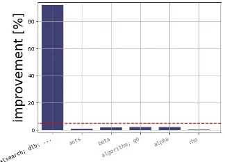
Fig. 2: Ablation analysis (with surrogate) on the path from ACOTSP default configuration to the best configuration returned by irace. The y-axis shows the percentage of performance gain when switching the value of each parameter.
It should be noted that the finding of fANOVA and ablation analysis on the most important parameters is not necessarily consistent in all cases. fANOVA analysis works on the whole configuration space, while ablation analysis focuses on the local path between two specific configurations. Therefore, the dominance of parameter localsearch given by both analyses emphasises the importance of this parameter on both the global and the local scale.
[image:6.595.230.392.353.470.2]3.2 Case study 2: tuning irace on a configuration benchmark
iraceis an automatic algorithm configurator, but it also has its own parameters. In [5], irace is used to configure irace on different configuration benchmarks in a procedure called meta-tuning. To avoid confusion, the higher-layer irace is named meta-irace. In an algorithm configuration setting, the tuned irace is simply considered as a parametrised optimisation algorithm, and each algorithm configuration benchmark plays the role of a problem instance. In this case study, we consider one of the meta-tuning experiments in [5], where irace is tuned on a configuration benchmark of the mixed-integer programming solverCPLEX [13], namelyCPLEX-REG, with a budget of 5000 irace runs. The tuned irace has 9 parameters, including 3 categorical parameters (elitist,testType,softRestart), 5 integer parameters (nbIterations,minNbSurvival,elitistInstances,mu,firstTest) and one continuous parameter (confidence). The default configuration of irace and the five best configurations returned by meta-irace are shown in Table 2. The improvement given by meta-irace over the default configuration is statistically significant (Wilcoxon signed rank test with a confidence level of 99%).
The aim of the analyses in this case study is to understand the choice of the configurator (here, meta-irace) on the best irace’s configurations. We will show that the interpretation of the analyses here is more complicated compared to the previous case study. In particular, the ablation analysis in the two di-rections can provide different results due to the complex interactions between irace’s parameters. Moreover, a complementary usage of various fANOVA pack-age’s functionalities to gain more insights into the findings given by the ablation analysis is also presented.
nbIterations minNbSurvival confidence elitist elitistInstances testType mu firstTest softRestart (Elite configurations)
35 2 0.52 false t-test-holm 4 6 true
29 1 0.55 false t-test-holm 4 5 true
37 1 0.51 false t-test-holm 4 5 false
29 1 0.55 false t-test-holm 3 5 true
12 1 0.77 false t-test 7 5 true
(Default configuration)
8 8 0.95 true 1 t-test 5 5 true
Table 2: irace’s default configuration and the five best configurations given by meta-irace.
Ablation analysis. Ablation in both directions between two algorithm config-urations was recommended [6]. The rationale for this is due to the possibility of interactions between parameters. This case study is a clear example of this situation. We will show that the reverse path can give interesting information that is not really obvious in the original path.
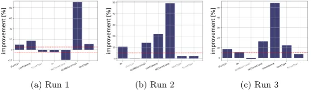
the parameters are chosen as well as their contribution on the performance gain vary quite a bit among different runs. This can be seen in the plots of three example paths shown in Figure 3. Because of those fluctuations, it is difficult to draw any conclusions from the ablation analysis in this direction.
[image:8.595.150.467.190.284.2](a) Run 1 (b) Run 2 (c) Run 3
Fig. 3: Three ablation paths from the irace default configuration to the best one returned by meta-irace.
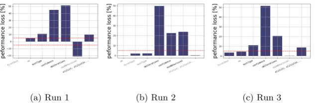
We apply another ten times the ablation, now on the reverse path from the best configuration to the default configuration. At each step, the parameter that introduces the least performance loss when changing its value from the best con-figuration to the default one is chosen. Figure 4 shows the reverse paths with the same random seeds as in the ones used in Figure 3. We can see that the orders in which the parameters are chosen along the paths are more consistent among different runs. In particular, the four parametersnbIterations,confidence, minNbSurvivalandelitist are always chosen at the end of the path, which means that changing their values in the best configuration will cause more performance loss than all other parameters. Indeed, most of the performance loss on the paths are due to the three parametersnbIterations,confidence,minNbSurvival. Param-eter elitist is constantly the last one chosen in the ten paths although it is not explicitly associated with a big loss in performance. This indicates two things: (i) the importance of setting this parameter at the right value for achieving the good performance of the best configuration, as changing its value in the path between the best configuration to the default one will induce larger performance loss than any other parameters, (ii) the strong dependency of this parameter and the others, especially the three parametersnbIterations,confidence, minNb-Survival; or, in other words, the possibly complicated interactions between these parameters in the local region between the two configurations under study.
(a) Run 1 (b) Run 2 (c) Run 3
Fig. 4: Three ablation paths from the best one returned by meta-irace the default irace configuration.
We do two fANOVA analyses, one on the global space, dubbedglobal-fANOVA and one on the local space where the algorithm performance is not worse than the default one, namely capped-fANOVA. Parts of them are shown in Table 3.
global-fANOVA capped-fANOVA
All single-parameter effects: 38.01% All single-parameter effects: 11.69% All pairwise interaction effects: 34.31% All pairwise interaction effects: 28.17% nbIterations: 11.8% firstTest x nbIterations: 3.89%
minNbSurvival: 6.22% minNbSurvival: 3.28%
firstTest: 5.73% firstTest x minNbSurvival: 2.82%
testType: 5.25% firstTest: 2.55%
confidence: 5.21% minNbSurvival x nbIterations: 2.26% ... (remaining effects:<4%) ... (remaining effects:<2%)
Table 3: Partial results of fANOVA analyses on irace’s performance data
The differences between the two analyses are that in the local one, single parameter effects become less important, both single parameter and pairwise interaction effects have less contribution to the total performance variance, and their contribution is more widely spread. One possible explanation for these differences is that in the local space, the interactions of algorithm parameters are more complicated. Anyway, one clear thing is thateliltist parameter is not among the top list effects in both analyses.
higher-order) interactions betweenelitistand the other three parameters is only 5.18%, and it generally is spread evenly among them. It means that there are no impor-tant interactions as expected. Since capped-fANOVA works on the configuration space where performance value is not worse than the default configuration, the observations in this analysis indicate that the importance ofelitist is even more local, i.e., it only works when not only the three parametersnbIterations, confi-dence,minNbSurvival are set properly, but also the other ones have to be in the appropriate ranges. In fact, if we look at the values of the other parameters in the default and the best configurations, we can see that they are already quite close to each other. For example, the parameterfirstTest has the values of 5 and 6 in the default and the best configurations, respectively, while its domain is [4,20]. We can further confirm our conjecture as follows. First, we ask fANOVA for the predicted average cost of the default and the best configurations (here we get 138.92 and 135.81). Next, we modify the value of parameter firstTest in the best configuration to a more distant one, say 12. Then we ask fANOVA for the predicted cost of this new configuration (here we get 138.78). This increasing cost implies the importance of havingfirstTest near the local region around 6.
In summary, the conclusion from this fANOVA analysis is that the impor-tance of irace parameters and the choice of the meta-irace are very local, i.e., al-though the four parameterselitist,nbIterations,confidence,minNbSurvivalplay essential roles in improving the performance between the default and the best configurations, the other parameters also need to be set in the appropriate ranges that are not far from their values indicated in the best configuration. Therefore, if irace’s developers want to explain what changes in irace’s behaviours (according to its parameters) make the performance improved, they will need to associate those changes with all parameters instead of only a few of them.
3.3 Case study 3: a Large Neighbourhood Search for a Vehicle Routing Problem with Time Windows
The example analyses so far are only on the algorithm configuration space. In this case study, we illustrate the integration of problem instance features into fANOVA analysis, so that we can study not only the impact of algorithm pa-rameters, but also their interactions with instance features.
fANOVA analysis. We can add instance features into fANOVA analysis by treating them as algorithm parameters, i.e., each combination of algorithm con-figuration and instance feature is given to fANOVA as an algorithm configura-tion. It must be noted that this integration can only be done when the instance features are independent, since this is one of the key assumptions fANOVA makes on its input variables. In this case study, the problem instances are generated based on random values drawn from all instance features in an independent way. A part of fANOVA’s output is given in the left column of Table 4.
On original performance data On normalised performance data All single-parameter effects: 80.87% All single-parameter effects: 60.74% All pairwise interaction effects: 12.23% All pairwise interaction effects: 15.38% customer number: 75.24% repair: 52.68%
average service time x customer number: 5.24% destroy x repair: 4.42%
average service time: 3.78% customer number x repair: 4.19% ... (remaining effects:<2%) customer number: 4.0%
destroy: 3.14%
... (remaining effects:<3%)
Table 4: Partial results of fANOVA analyses on LNS algorithm performance data
[image:11.595.225.393.503.632.2]An obvious observation from this result is that only instance features are listed as the most important variables. In particular, the featurecustomer number has a clear dominant influence, as it explains 75.24% of the total performance variance. Looking at its marginal plot shown in Figure 5, we can see that the av-erage performance values increase according to this feature. This means that the range of the algorithm performance values greatly depends on problem instance size (here it is the number of customers).
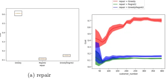
In situations like this, depending on the aim of our analysis, normalisation can be necessary. Here we aim to study the algorithm performance without any bias towards particular instances, which is similar to what irace’s default setting does as described in section 3.1. Therefore, we re-run the fANOVA analysis, now with normalised performance values. A part of the new results is listed in the right column of Table 4. The impact of customer number is now significantly reduced, so that the influence of algorithm parameters becomes visible. The two categorical algorithm parametersrepairanddestroy, which represent the choices of the repair and the destroy operators inside the Large Neighbourhood Search, now involves in the top list of important parameters and pairwise interactions. In particular, the high contribution percentage of parameterrepair (52.68%) on the total performance variance and its marginal plot (Figure 6a) show that the repair operators Regret2 and Greedy work generally best and worst, respectively, across the whole problem instance space. In addition, we can also see how much influence the choice is according to different problem sizes by looking at the marginal plot of the pairwise interactionrepair xcustomer number (Figure 6b): on instances with the number of customers less than 50, the bad performance of Greedy is not as obvious as on instances with larger sizes; for the other two choices, Regret2 and GreedyRegret2, their overall performance difference also gets clearer when the number of customers increases. Other problem instance features do not have important interactions with algorithm parameters.
(a) repair
[image:12.595.139.413.393.526.2](b) customer number x repair
Fig. 6: Marginal plots of the algorithm parameter repair and its pairwise inter-action with the instance feature customer number given by fANOVA analysis with performance normalisation.
such an analysis, in this case study, takes a large amount of time to run (16 hours on a single core Intel CPU 2.4Ghz) 3. The reason is due to the heavy computation of all pairwise interactions. In this part, we demonstrate a cheaper alternative for this particular case using a combination of fANOVA and forward selection. First, we use fANOVA to calculate the importance of single variables. Next, we use forward selection to identify the key subset of variables, and then use fANOVA to examine interactions of the variables in that set only. In this way, the whole analysis takes less than half an hour.
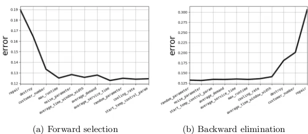
First, we apply fANOVA on single parameter effects only, which takes less than one minute to finish. Next, we apply forward selection to the normalised performance dataset. Since analysis results might vary among different runs, we repeat it ten times. It takes about 3 minutes in total. The visualisation of one run’s result, which is a path of sequentially adding one variable to the model at a time so that the resulting root mean square error on the validation set is minimised, is shown in Figure 7a. We can see that the first three parameters chosen arerepair,destroy andcustomer number. This happens to be the case for all the ten runs; these three parameters are always chosen first, while the fourth parameter onwards in the path can vary among different runs. This indicates the high relevance of these three parameters on the prediction model.
Since these experiments are computationally cheap, we also apply backward elimination, the reverse procedure of forward selection, where starting from the whole variable set, one variable resulting the least decrease in the prediction error is removed sequentially. This may help to take into account dependency between the parameters. These runs take about 5 minutes in total. The chosen path and the error values in one of the ten runs is shown in Figure 7b. The three parameters repair,destroy and customer number are the last one to be chosen, and this is again consistent among the ten runs. This implies the importance of these parameters’ interactions.
Given those indications, we can now focus on analysing the interactions be-tween these three variables using fANOVA. Results of the importance quan-tification and marginal plots given the three variables repair, destroy and cus-tomer number are obviously the same as the original fANOVA, with an addition of the three-way interaction between those variables. However, since the impor-tance of this interaction is rather small (2.3%), we can simply ignore it. This particular fANOVA analysis takes about two minutes. So the whole analysis only needs 12 minutes.
4
Conclusions and future work
In this paper, we have demonstrated and discussed the complementary usage of three parameter analysis techniques, namely forward selection [9], fANOVA [10] and ablation [6, 2] analyses. This is done using three case studies, each of which
3
(a) Forward selection (b) Backward elimination
Fig. 7: Prediction error of the model trained on a subset of variables chosen during one run of forward selection and backward elimination analyses.
represents some special situations that the analyses can fall into. In the first and the second case study, where the aim is to use fANOVA and ablation analyses to understand the choice of the best configuration given by an automatic algo-rithm configuration tool (here irace), analysis conclusions diverge: in the first one, there is a dominant parameter in both the global configuration space and the local space between the default and best algorithm configurations, so that the algorithm developers can focus on this particular parameter for explaining the improvement over the default configuration; in the second one, the impact of parameters are very local and the algorithm performance improvement gained re-quires all parameters to be in their reasonable ranges of values, which means that the developers need to look at all parameter values as a whole instead of focusing on a few of them. In the third case study, the integration of problem instance features into fANOVA analysis is illustrated. This shows how the range of al-gorithm performance values changes according to problem instance sizes; hence, it emphasises the necessity of normalising performance data to avoid bias. The interaction between algorithm parameters and instance features also provides interesting insights into how the impact of important algorithm parameters can vary among different problem sizes. Moreover, a complementary usage of the forward selection analysis that can help to significantly reduce the computation cost of fANOVA analysis in this particular case study is also presented.
Acknowledgement This work is funded by COMEX (Project P7/36), a BEL-SPO/IAP Programme. The computational resources and services were provided by the VSC (Flemish Supercomputer Center), funded by the Research Founda-tion - Flanders (FWO) and the Flemish Government - department EWI. The authors are grateful to Thomas St¨utzle and the anonymous reviewers for their valuable comments, which help to improve the quality of the paper.
References
1. Bartz-Beielstein, T., Lasarczyk, C., and Preuss, M.The sequential parame-ter optimization toolbox. InExperimental Methods for the Analysis of Optimization Algorithms, T. Bartz-Beielstein, M. Chiarandini, L. Paquete, and M. Preuss, Eds. Springer, Berlin, Germany, 2010, pp. 337–360.
2. Biedenkapp, A., Lindauer, M., Eggensperger, K., Hutter, F., Fawcett, C., and Hoos, H. H. Efficient parameter importance analysis via ablation with
surrogates. InAAAI Conference on Artificial Intelligence (Feb. 2017), S. P. Singh and S. Markovitch, Eds., AAAI Press.
3. Chiarandini, M., and Goegebeur, Y. Mixed models for the analysis of op-timization algorithms. Experimental Methods for the Analysis of Optimization Algorithms 1 (2010), 225.
4. Corstjens, J., Caris, A., Depaire, B., and S¨orensen, K.A multilevel method-ology for analysing metaheuristic algorithms for the VRPTW.
5. Dang, N., P´erez C´aceres, L., De Causmaecker, P., and St¨utzle, T. Con-figuring irace using surrogate configuration benchmarks. In Proceedings of the Genetic and Evolutionary Computation Conference (2017), ACM, pp. 243–250. 6. Fawcett, C., and Hoos, H. H. Analysing differences between algorithm
config-urations through ablation. Journal of Heuristics 22, 4 (2016), 431–458.
7. Hooker, G. Generalized functional ANOVA diagnostics for high-dimensional functions of dependent variables. J. Comput. Graph. Stat 16, 3 (2012), 709–732. 8. Hutter, F., Hoos, H. H., and Leyton-Brown, K. Sequential model-based
optimization for general algorithm configuration. InLION 5, C. A. Coello Coello, Ed., vol. 6683 ofLNCS. Springer, Heidelberg, 2011, pp. 507–523.
9. Hutter, F., Hoos, H. H., and Leyton-Brown, K.Identifying key algorithm pa-rameters and instance features using forward selection. InLION7 (2013), Springer, pp. 364–381.
10. Hutter, F., Hoos, H. H., and Leyton-Brown, K.An efficient approach for as-sessing hyperparameter importance. InProc. of the 31th International Conference on Machine Learning (2014), vol. 32, pp. 754–762.
11. Hutter, F., Hoos, H. H., Leyton-Brown, K., and St¨utzle, T. ParamILS: an automatic algorithm configuration framework. J. Artif. Intell. Res 36 (Oct. 2009), 267–306.
12. Hutter, F., Xu, L., Hoos, H. H., and Leyton-Brown, K. Algorithm runtime prediction: Methods & evaluation. Artificial Intelligence 206 (2014), 79–111. 13. IBM. ILOG CPLEX optimizer. http://www.ibm.com/software/integration/
optimization/cplex-optimizer/, 2017.
14. L´opez-Ib´a˜nez, M., Dubois-Lacoste, J., P´erez C´aceres, L., St¨utzle, T., and Birattari, M. The irace package: Iterated racing for automatic algorithm configuration. Operations Research Perspectives 3 (2016), 43–58.