Application of Structured Total Least Squares for
System Identification and Model Reduction
Ivan Markovsky, Jan C. Willems, Sabine Van Huffel, Bart De Moor, and Rik Pintelon
, Fellow, IEEE
Abstract—The following identification problem is considered: Minimize the 2norm of the difference between a given time series and an approximating one under the constraint that the approxi-mating time series is a trajectory of a linear time invariant system of a fixed complexity. The complexity is measured by the input dimension and the maximum lag. The question leads to a problem that is known as the global total least squares problem and alter-natively can be viewed as maximum likelihood identification in the errors-in-variables setup. Multiple time series and latent variables can be considered in the same setting. Special cases of the problem are autonomous system identification, approximate realization, and finite time optimal 2 model reduction. The identification problem is related to the structured total least squares problem. This paper presents an efficient software package that implements the theory. The proposed method and software are tested on data sets from the database for the identification of systems DAISY.
Index Terms—DAISY, errors-in-variables, model reduction, MPUM, numerical software, system identification, structured total least squares.
I. INTRODUCTION
A. The Structured Total Least Squares Problem
T
HE structured total least squares (STLS) problem orig-inates [1], [2] from the signal processing and numerical linear algebra communities and is not widely known in the area of systems and control. It is a generalization to ma-trices with structure of the total least squares problem [3], [4] known in the early system identification literature as theManuscript received May 26, 2004; revised January 27, 2005 and May 31, 2005. Recommended by Guest Editor L. Ljung. The work of I. Markovsky was supported by a K.U. Leuven doctoral scholarship. Research was supported by:
Research Council KUL: GOA-Mefisto 666, GOA-Ambiorics, IDO/99/003
and IDO/02/009 (Predictive computer models for medical classification problems using patient data and expert knowledge), several Ph.D./postdoctoral and fellow grants;Flemish Government: FWO:Ph.D./postdoctoral grants, projects, G.0078.01 (structured matrices), G.0269.02 (magnetic resonance spectroscopic imaging), G.0270.02 (nonlinear Lp approximation), G.0240.99 (multilinear algebra), G.0407.02 (support vector machines), G.0197.02 (power islands), G.0141.03 (Identification and cryptography), G.0491.03 (control for intensive care glycemia), G.0120.03 (QIT), G.0452.04 (QC), G.0499.04 (robust SVM), research communities (ICCoS, ANMMM, MLDM); AWI: Bil. Int. Collaboration Hungary/Poland; IWT:Ph.D. Grants; GBOU (McKnow)
Belgian Federal Government:DWTC (IUAP IV-02 (1996–2001) and Belgian
Federal Science Policy Office IUAP V-22 (2002–2006) (Dynamical Systems and Control: Computation, Identification and Modeling)); PODO-II (CP/01/40: TMS and Sustainibility); EU: PDT-COIL, BIOPATTERN, eTUMOUR, FP5-Quprodis; ERNSI; Eureka 2063-IMPACT; Eureka 2419-FliTE; Contract Research/agreements: ISMC/IPCOS, Data4s, TML, Elia, LMS, IPCOS, Mastercard.
I. Markovsky, J. C. Willems, S. Van Huffel, and B. De Moor are with the Electrical Engineering Department, K. U. Leuven, B-3001 Leuven, Belgium (e-mail: [email protected]).
R. Pintelon is with Department ELEC, Vrije Universiteit Brussel, B-1050 Brussels, Belgium.
[image:1.594.320.538.163.268.2]Digital Object Identifier 10.1109/TAC.2005.856643
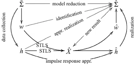
Fig. 1. Different problems aiming at a (low complexity) model 6^ that approximates a given (high complexity) model6. The time serieswis an observed response andhis an observed impulse response.
Koopmans–Levin’s method [5]. In this paper, we show the applicability of the STLS method for system identification. We extend previous results [6], [7] of the application of STLS for single-input–single-output (SISO) system identification to the multiple-input–multiple-output (MIMO) case and present numerical results on data sets from DAISY [8].
The STLS problem is defined as follows: Given a time series and a structure specification , find the global minimum point of the optimization problem
subject to (1)
The constraint of (1) enforces the structured matrix to be rank deficient, with rank at most . The cost function measures the distance of the given data to its approximation . Thus the STLS problem aims at optimal structured low rank
approximation of by .
B. Approximate Modeling Problems
Fig. 1, shows several approximate modeling problems. On top is the model reduction problem: given alinear time-invariant
(LTI) system , find an LTI approximation of a desired lower complexity. A tractable solution that gives very good results in practice is balanced truncation [9]. We consider finite time optimal model reduction: The sequence of the first Markov parameters of is approximated by the sequence of the corre-sponding Markov parameters of in the norm sense.
The identification problem is similar to the model reduction one, but starts instead from an observed response . Various data collection models (the down arrows from to and in Fig. 1) are possible. For example, theerrors-in-variablesmodel: , where is a trajectory generated by and is measurement noise.
Of independent interest are the identification problems from an observed impulse response , calledapproximate realization
problem, and the autonomous system identification problem, where and are free responses. A classical solution to these problems is Kung’s algorithm [10].
The key observation that motivates the application of STLS for system identification and model reduction is that their kernel subproblem is to find a block-Hankel rank deficient matrix approximating a given full-rank matrix with the same structure. Methods like balanced model reduction, subspace identification, and Kung’s algorithm solve the kernel problem via the singular value decomposition (SVD). For finite matrices, however, the SVD approximation of is unstructured. For this reason the algorithms based on the SVD are suboptimal with respect to an induced norm of the residual . The STLS method, on the other hand, preserves the structure and is optimal according to this criterion. Our purpose is to show how system theoretic problems with misfit optimality criterion are solved as equivalent STLS problems and subsequently make use of efficient numerical methods developed for the STLS problem [11]–[13].
C. The Global Total Least Squares Problem
Let be a user specified model class and let be an ob-served time series of length . We view a model
as a collection of legitimate time series. The more the model forbids from the universe of possible time series, the less com-plex and therefore more powerful it is. The model class restricts the maximal allowed model complexity. Within , we aim to find the model that best fits the data according to the misfit criterion
with
The resulting optimization problem is known as theglobal total least squares(GTLS) problem [14]. The described system iden-tification framework is put forward in [15].
The approach of Roorda and Heij [14], [16] is based on solving the inner minimization problem, the misfit computa-tion, by using isometric state representation and subsequently used alternating least squares or Gauss–Newton type algorithm for the outer minimization problem. They use a state space representation with driving input. Our approach of solving the GTLS problem, is different. We relate the identification problem to the STLS problem (1) and subsequently use solution methods developed for the STLS problem. Also we use a kernel representation of the system.
D. Link With the Most Powerful Unfalsified Model
In [17], the concept of themost powerful unfalsified model
(MPUM) is introduced. A model is unfalsified by the obser-vation if . A model is more powerful than if . Thus the concept of the MPUM is to find the most powerful model consistent with the observations—a most rea-sonable and intuitive identification principle.
In practice, however, the MPUM could be unacceptably com-plex. For example, in the errors-in-variables setup the
observa-tion w, is perturbed by noise,
so that with probability one the MPUM is all of w . Such a model is useless because it imposes no laws.
The GTLS problem addresses this issue by restricting the model complexity by the constraint , where is an
a priorispecified model class. Whenever the MPUM does not belong to , an approximation is needed. The idea is to modify as little as possible the given time series, so that the MPUM of the modified time series belongs to —a most reasonable gen-eralization of the MPUM to the bounded complexity case. The measure of closeness is chosen as the norm, which weights equally all variables over all time instants. Weighted norms can be used in order to take into account prior knowledge about nonuniform variance among the variables and/or in time.
E. Outline of this Paper
Section II gives background material on LTI systems de-scribed by kernel representation. Section III defines and solves the identification problems. Section IV describes some exten-sions of the identification problem. Section V describes the special identification problems from impulse and free response. Section VI shows results of the proposed method on data sets from DAISY, and Section VII gives conclusions.
II. PRELIMINARIES
A. Kernel Representation
Consider a time series . The
block-Hankel matrix with block rows, constructed from the time se-ries , is denoted by
..
. ... ...
The time series satisfies the set of difference equations
for (2)
with maximum lags(i.e., unit delays in time), if and only if
where
The rank deficiency of is related to the existence of an LTI system that “explains” the data and the Hankel structure is related to the dynamic nature of the model.
In the behavioral approach to system theory [18], (2) is called akernel representationof the system . A more compact nota-tion is
where (3)
and is the backward shift operator, . Let be the set of all trajectories of a system , described by (3), i.e.,
w
We identify thebehavior of with the system itself. No
B. Shortest Lag Representation
A kernel representation (3) for a given is not unique. If the polynomial matrix defines a kernel representation of ,
then for any unimodular matrix also
defines a kernel representation of . The kernel representation is called minimal if is full row rank. There exists a minimal one, calledshortest lag representation [19, Sec. 7], in which the number of equations , the maximum lag , and the total lag , where is the lag of the th equation, are all minimal. A kernel representation
is a shortest lag representation if and only if is row proper. Let be the degree of the th row of . The polynomial matrix is calledrow properif the leading row coefficient matrix, i.e., the matrix of which the th entry is the coefficient of the term with power of , is full row rank.
In a shortest lag representation the number of equations is equal to the number of outputs in an input/output representation and the total lag is equal to the state dimension in a minimal state–space representation. These numbers areinvariantsof the system; see [19, Sec. 4]. The maximal lag of , denoted by , is called the lag of the system, and its total lag, denoted by , is called the order of the system.
C. Model Class
The number of inputs and the number of outputs in an input–output or input/state/output representation are also invariants of the system . We denote by the set of LTI systems with inputs and lag at most . (Occasionally, we dis-play the number of variables as follows w .) The natural numbers and specify the maximum complexity of a model in the model class . For and sufficiently large, the restriction of the behavior to the interval has
dimension .
The specification of the complexity by the lag of the system does not fix the order, i.e., the minimal state dimension. For a system , the order of is in the range
.
In Section V, we use the notation for the input/state/output representation
(4)
of the LTI system such that (4) holds .
The column vector with (block) entries is denoted
by .
III. IDENTIFICATION IN THEMISFITSETTING BYSTLS The considered identification problem is defined as follows.
Problem 1(GTLS): For given time series and a complexity specification , where is the number of inputs and is the lag of the identified system, solve the optimization problem
(5)
The optimal approximating time series is , corresponding to a global minimum point of (5), and the optimal approximating system is .
Problem 1 is the GTLS problem for the model class . The inner minimization problem, i.e., the misfit
computation, has the system theoretic meaning of finding the best approximation of the given time series , that is a trajec-tory of the (fixed from the outer minimization problem) system
. This is asmoothing problem.
Our goal is to express (5) as an STLS problem (1).
There-fore, we need to ensure that the constraint is
equivalent to . As a byproduct of doing this, we relate the parameter , in the STLS problem formulation, to the system . The equivalence is proven under an assumption that is conjectured to hold generically in the data space w .
Lemma 1: Consider a time series
w, and natural numbers and . Assume
that for certain matrix
w, where , with being full row
rank. Then the system , defined by the kernel
represen-tation with , is such that
, and the order of is .
Proof: By definition is a linear system with lag . The assumption that is full-row rank implies that is row proper. Then the number of outputs of is
and, therefore, . This proves
that .
Let be the degree of the th equation in . The assumption that is full row rank implies that for all .
Therefore, .
Finally, implies , for
, so that .
The next lemma states the reverse implication.
Lemma 2: Consider a time series
w
and natural numbers and . Assume that there is
a system with order , such that .
Let , where , be a shortest lag
kernel representation of . Then, is full-row rank and the
matrix annihilates the Hankel matrix
, i.e., .
Proof: Let be the degree of the th equation in
. We have and . The assumption
is possible only if , for all . Because is row proper (by the shortest lag assumption of the kernel representation), the leading row coefficient matrix has full-row rank. But since
, for all .
The fact that follows from .
We have the following main result.
Theorem 1: Assume that is a system that admits a kernel representation
with of full-row rank. Then,
the constraint is equivalent to the constraint
, where .
property. In the direction of assuming , by Lemma 2, it follows that . Since is of full-row rank,
is equivalent to , with
. In the opposite direction, by
Lemma 1, with
. Therefore, is of full-row rank.
Theorem 1 states the desired equivalence of the GTLS problem and the STLS problem under the assumption that the optimal approximating system admits a kernel representation
with full row rank (6)
We conjecture that (6) holds true for almost all w . Define the subset of w consisting of all time series
w for which the GTLS problem is equivalent to the STLS problem, i.e.,
w Problem (5) has a unique global minimizer that satisfies (6)
Conjecture 1: The set is generic in w , i.e., it contains an open subset, whose complement has measure zero.
The existence and uniqueness part of the conjecture (see the definition of ) is justified in [20, Sec. 5.1]. The justification for (6) being generic is the following one. The highest possible order of a system in the model class is . One can ex-pect that generically in the data space w . By Lemma 2, implies that in a kernel representation is of full row rank. But generically in
the matrix , defined by , is
of full-row rank. Although the justification for the conjecture is quite obvious, the proof seems to be rather involved.
A. Properties of the Solution
The following are properties of the smoothing problem: i) is orthogonal to the correction , and ii) is generated by an LTI system . Since the GTLS problem has as an inner minimization problem, the smoothing problem, the same properties hold in particular for the optimal solution of (5). These results are stated for the SISO case in [6] and then proven for the MIMO case in [14, Sec. VI].
Statistical properties of the GTLS problem, are studied in the literature. For the stochastic analysis, the errors-in-variables model is assumed and the basic results are consistency and asymptotic normality. Consistency in the SISO case is proven in [21]. Consistency in the MIMO case is proven in [20], in the framework of the GTLS problem. Complete statistical theory with practical confidence bounds is presented in [22], in the setting of the Markov estimator for semilinear models. Consistency of the STLS estimator for the general structure specification described in Appendix A is proven in [23].
B. Numerical Implementation
A recursive solution of the smoothing problem
is obtained by dynamic programming in [24]. An alternative derivation by isometric state representation is given in [14]. Both solutions are derived from a system theoretic point of view. A related problem occurs in the STLS formulation, where it is viewed from a numerical linear algebra point of view and is solved in a different way.
Because of the flexible structure specification, the inner min-imization problem in the STLS formulation (1) is more general than the smoothing problem, where the block-Hankel structure is fixed. A closed form expression is derived and a special struc-ture of the involved matrices is recognized, see [12] for details. The structure is then used on the level of the computation by employing numerical linear algorithms for structured matrices [25]. The resulting computational complexity is linear in the length of the given time series .
The outer minimization problem ,
how-ever, is a difficult nonconvex optimization problem that requires iterative methods. Two methods are proposed in the frame-work of the GTLS problem. In [14], an alternating least squares method is used. Its convergence is linear and can be very slow in certain cases. In [16], a Gauss–Newton algorithm is proposed. For the solution of the STLS problem, a Levenberg-Marquardt algorithm is used. More details on the implementation of the latter algorithm can be found in Appendix A, where a software package for solving the STLS problem (1) is described. The convergence of all these algorithms to the desired global min-imum is not guaranteed and depends on the provided initial approximation and the given data.
IV. EXTENSIONS
A. Input/Output Partitionings
A standard assumption in system identification is that an input/output partitioning of the variables is a priori given. Consider a permutation matrix and redefine as . The first variables of the redefined time series are assumed to be inputs and the remaining variables outputs.
With and , the kernel
representation becomes aleft matrix fraction rep-resentation . The transfer function of for the
fixed by input/output partitioning is .
Let with squares. Under the assumption
, the state–space representation
. .. ... ...
is minimal. Therefore, the transition from and (which is the result obtained from the STLS optimization problem) to an input/state/output representation is trivial and requires extra computations only for the formation of the matrix.
. Moreover, we conjecture that generically admits an arbitrary input–output partitioning (i.e., , with any permutation matrix ).
B. Exact Variables
Another standard assumption is that the inputs are exact (in the errors-in-variables context noise free). Let and be the estimated input and output. The assumption that is exact im-poses the constraint .
More generally, if some variables of are exact, then the corresponding elements in are fixed. In the STLS problem formulation (1), the exact elements of can be separated in a block of by permuting the columns of . The software package described in Appendix A allows specification of exact blocks in that are not modified in the solution . After solving the modified problem, the solution of the original problem, with exact variables, is obtained by applying the reverse permutation.
With a given input–output partition (defined by a permutation matrix ) and exact inputs, the GTLS problem becomes the output error identification problem
In Problem 5, the approximating trajectory isanytrajectory of , while in the output error identification problem, the approxi-mating trajectory is generated by thegiveninput and only the initial conditions are freely chosen. In the single output, output error identification problem, the misfit
subject to
is equivalent to the cost function minimized by the prediction error methods. Simulation results are shown in Section VI-A.
C. Multiple Time Series
In certain cases, e.g., the noisy realization problem, not one but several observed time series are given. Assume that all time series are of the same length and define to be the matrix valued time series , so that
. The only modification needed for this case is to consider block-Hankel matrix with size of the blocks instead of , as for the case of a single observed time series. The software package described in Appendix A can deal with such problems.
D. Known Initial Conditions
In the GTLS problem, no prior knowledge about initial con-ditions is assumed. Thus, the best fitting trajectory is searched in the whole behavior of the approximating system. If the ini-tial conditions are a priori known, should be searched only among the trajectories of , generated with the specified initial conditions. A typical examples of identification problems with known initial conditions are approximate realization and identi-fication from step response observations. In both cases, the ini-tial conditions area prioriknown to be zero.
Fig. 2. Example of an autonomous identification problem in the errors-in-variables setting. Solid line—exact trajectoryy, dotted line—datay, dashed line—approximating trajectory^y.
Zero initial conditions can be taken into account in the iden-tification problem by extending the given time series with zero samples. Let be the obtained in this way extended data sequences. In order to ensure that the approximation is also obtained under zero initial conditions, the first samples of should be preserved unmodified in .
Note 1: In the current software implementation of the GTLS method the specification that the leading data samples are exact isnotpossible. This feature of the identification problem goes beyond the scope of the current STLS solution method and soft-ware.
E. Latent Inputs
The classical system identification framework [26] differs from the one in this paper in the choice of the optimization criterion and the model class. In [26], an unobserved input
is assumed to act on the system that generates the observations and the optimization criterion is defined as the prediction error.
The unobserved input , calledlatent input, plays the role of innovations. Written in a polynomial form, the model with latent inputs is the classical ARMAX model
Latent input can be accommodated in the setting of Section III, by augmenting the model class with extra inputs and the cost function with the term . The re-sulting identification problem is
subject to
It unifies the misfit and latency description of the uncertainty and is put forward by Lemmerling and De Moor [7]. The pure latency identification problem
subject to (8)
corresponds to the prediction error approach.
The misfit-latency identification problem (7) can easily be re-formulated as an equivalent pure misfit identification problem
(5). Let , where is an
-dimen-sional zero time series. Then, the misfit minimization problem for the time series and the model class is equiva-lent to (7). The pure latency identification problem (8) can also be treated in our framework by considering exact (see Sub-section IV-B) and modifying only . Note that the latent input amounts to increasing the complexity of the model class, so that a better fit is achieved with a less powerful model.
V. SPECIALPROBLEMS
In this section, we consider three special identification prob-lems in an input/output setting. In the first one the data is an observed impulse response. In the second one the data is an ob-served free response. In the third one, the data is an exact im-pulse response of a high order system, i.e., a system that is not in the specified model class.
A. Approximate Realization
Identification from exact impulse response is the topic of (par-tial) realization theory. When the given data
(impulse response observations) is not exact, an approximation is needed. Kung’s algorithm is a well known solution for this problem. However, Kung’s algorithm is suboptimal in terms of the misfit criterion
where
is an impulse response of
The GTLS problem can be used to find optimal in terms of the misfit approximate model.
Problem 2 (Approximate realization [27]): Given a matrix valued time series and a natural number ,
solve the optimization problem .
The approximate realization problem is a special GTLS problem and can be treated as such. Now, however, the given matrix valued trajectory is an observed impulse response, so that the input is a pulse and the initial conditions are zeros. For this reason the direct approach is inefficient. In the rest of this section, we describe an indirect solution that exploits the special features of the data.
The following statement is a corollary of Theorem 1.
Corollary 1: Consider a shortest lag kernel representation
(i.e., row proper) and define , where is
square. If is nonsingular, then is an impulse
response of if and only if , where
Corollary 1 shows that under assumption (6), the approximate realization problem can be solved as an STLS problem with structured data matrix . Next we specify how one can obtain an input/state/output representation of the optimal approximating system from and the
approxi-mated Markov parameters .
By Corollary 1, . Let
be a rank revealing factorization. Since is an impulse response of and must be of the form
(The basis of the representation is fixed by the rank revealing factorization.) We have
so that
However, . On the other hand
so that . Therefore a basis for
the null space of defines an observability matrix of , from which and can be obtained up to a similarity transformation. is the unique solution of the system
and .
Example 1 (Approximate realization): Consider a simulation example in the errors-in-variables setup, i.e., the data
is obtained as a noise corrupted impulse response of an LTI system . The time horizon is and the the additive noise standard deviation is 0.25. The true system is random stable (obtained via MATLAB’s function) with inputs, outputs, and lag . The approximate model is searched in the model class .
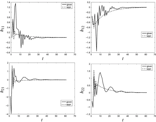
Fig. 3. Example of a finite time` model reduction problem. Solid line—impulse response of the given (high-order) system, dashed line—impulse response of the reduced order system.
0.2716 and in the second case 0.2608. (The difference is due to the wrong treatment, see Note 1, of the initial conditions in the direct method.) For comparison, the relative error with respect to the data is 0.9219.
B. Identification of an Autonomous System
The autonomous system identification problem is a special case of the GTLS problem when the model class is —the set of autonomous systems with lag at most .
Problem 3 (Autonomous System Identification): Given a time series and a natural number , find a system and a free response of , such that minimizes the approximation error over all free responses of systems in the model class .
It is easy to reformulate Problem 3 as a special case of the approximate realization problem. The shifted impulse response of the system is equal to the free response of the system , obtained under initial condition . Therefore, Problem 3 can be solved as an approximate realiza-tion problem with the obvious substiturealiza-tion. One can consider in the same way autonomous system identification for multiple
time series .
Example 2 (Identification of an autonomous system): Consider the same simulation setup as in Ex-ample 1 with the only difference that the true data is a single free response of length , obtained under random initial condition. The relative error of approximation is 0.4184 versus 0.7269 for the given data . Fig. 2, shows the fitting of by .
C. Finite Time Model Reduction
The finite time norm of a system with an impulse response is defined as
For a strictly stable system is well defined and is equal to its norm.
TABLE I
EXAMPLESFROMDAISY.T—TIMEHORIZON,m—NUMBER OFINPUTS,
p—NUMBER OFOUTPUTS,l—LAG
a system in the model class .) Then, the approximate re-alization problem can be interpreted as the following finite time
model reduction problem.
Problem 4 (Finite Time Model Reduction): Given a system , a natural number , and a time horizon , find a system , that minimizes the finite time
norm of the error system.
In the model reduction problem, the misfit is due to the low order approximation. In the approximate realization problem, assuming that the data is generated by an errors-in-variables model, the misfit is due to the measurement error . The so-lution methods, however, are equivalent, so in this section we actually give an alternative interpretation of the approximate re-alization problem.
Example 3 (Finite Time Model Reduction): The high-order system is a random stable system (obtained via MATLAB’s function ) with inputs,
outputs, and lag . A reduced-order model with lag is searched. The time horizon is chosen large enough for a sufficient decay of the impulse response of . (It is selected automatically by MATLAB’s function .)
Fig. 3 shows the fitting of the impulse response of the high-order system by the impulse response of the reduced-order system .
VI. PERFORMANCE ONDATASETSFROMDAISY The data base for system identification DAISY [8] is used for verification and comparison of identification algorithms. In this section, we apply the GTLS method, described in the paper and implemented by the software, presented in Appendix A, on data sets from DAISY. In Section VI-A, we solve output error identi-fication problems and in Section VI.B, we consider the data set “Step response of a fractional distillation column,” which con-sists of multiple vector time series.
A. Single Time Series Data Sets
The considered data sets are listed in Table I. Since all data sets are with a given input/output partitioning, the only user de-fined parameter that selects the complexity of the model class
is the lag .
The data is detrended and split into identification and valida-tion data sets. The first 70% of the data, denoted by , is used for identification, and the remaining 30%, denoted by , is used for validation.
Approximate models are computed via the following methods:
• the N4SID method implemented in the System Identification Toolbox of MATLAB;
TABLE II
COMPARISON OF THEMODELSOBTAINED BYn4sid,gtls,ANDpem
• the GTLS method implemented by the STLS solver;
• the prediction error method of the System Identi-fication Toolbox of MATLAB.
The inputs are assumed exact, so that identification in the output error setting is considered. The validation is performed in terms of the misfit obtained on the validation data set and the simulation fit computed by the function from the System Identification Toolbox.
so that these two criteria are equivalent.
Note 2 (About the Usage of the Methods): The function is called with the option
which specifies output error model structure. In addition, the options
and are used to disable the default for feedthrough term set to zero, robustification of the cost function, and sta-bility constraint. (The GTLS method does not constrain the model class by enforcing stability.) With these options (for the single output case) minimizes the output error misfit . The function is called with the specification that the inputs are exact, so that the GTLS and PEM methods solve equivalent identification problems. For both functions, we
set the same convergence tolerance ,
maximum number of iterations , and initial approximation (the model obtained by .
The identified systems by , , and are com-pared in Table II. In all examples there is a good match between the models obtained with the and functions. In ad-dition, the output error optimal model outperforms the model computed by the N4SID method. Since the criterion is checked on a part of the data that is not used for identification, there is noa prioriguarantee that this will be the case.
B. Identification From Step Response Measurements
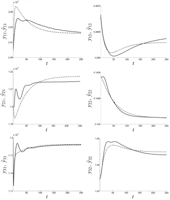
indepen-Fig. 4. Identification from step response measurements. Solid line—given datay, dashed line—GTLS approximation^y. (y is the step response from inputito outputj.)
dent time series, each one with data points. The given data has a fixed input/output partitioning with inputs and outputs. We further bound the complexity of the model class by choosing the lag , so that an approximate model is searched in the model class .
The step response data is special because, it consists of mul-tiple time series, the input is exactly known, and the initial con-ditions are also exactly known. In order to take into account the known zero initial conditions, we precede the given time series with zero samples. In order to take into account the exactly known inputs, we use the modification of the GTLS method for time series with exact variables. Multiple time series are pro-cessed as explained in Section IV.
Fig. 4 shows the given data (the measured step responses) with superimposed on them the step responses of the optimal approximating system, computed by the GTLS method.
VII. CONCLUSION
We generalized previous results on the application of STLS for system identification, approximate realization, and model
reduction to multivariable systems. The STLS method allows to treat identification problems, without input/output partitioning of the variables and errors-in-variables identification problems. Multiple time series, latent variables, and prior knowledge about exact variables can be taken into account.
A robust and efficient software tool for solving STLS prob-lems is presented. It makes the proposed identification method and its extensions practically applicable. The performance of the software package is tested on data sets from DAISY. The results show that examples with a few thousands data points and low order model can be solved routinely.
APPENDIX
A. Software Package for Solving STLS Problems [13]
[image:9.594.126.469.65.470.2]cubic computational complexity and are restricted to rank re-duction of order one. Thus, they are applicable only for small size SISO problems.
The described package solves the STLS problem (1) with , where is block-Toeplitz , block-Hankel , unstructured , or exact . All block-Toeplitz/Hankel structured blocks have blocks elements of the same row dimension .
The structure of is specified by and the array that describes the structure of the blocks specifies the block by giving its type , the number of columns , and (if is block-Hankel or block-Toeplitz) the column dimension of a block ele-ment. The input data for the problem is and the structure specification and .
The package uses MINPACK’s Levenberg–Marquardt algo-rithm to solve the optimization problem (1) in its equivalent for-mulation, see [11]
where
The weight matrix is block-Toeplitz and block-banded struc-tured, see [12], and this structure is exploited in the cost func-tion and first derivative evaluafunc-tion. There is no closed form ex-pression for the Jacobian matrix , where
, so that the pseudo-Jacobian proposed in [29] is used instead of . The cost function and pseudo-Jacobian evaluation is performed with computational complexity .
The software is written in ANSI C language. For the vector-matrix manipulations and for a C version of MIN-PACK’s Levenberg-Marquardt algorithm, the GNU Scientific library (GSL) is used. The computationally most intensive step of the algorithm—the Cholesky decomposition of the block-Toeplitz, block-banded weight matrix —is per-formed via the subroutine from the SLICOT library [30]. MATLABinterface via C-mex file is available.
An interface to the STLS solver for the purpose of approxi-mate system identification is developed in [31]. The MATLAB
implements the mapping ,
where is a GTLS optimal model. The function works with data consisting of multiple time series of equal length and allows for specification of exact variables. The soft-ware is available from http://www.esat.kuleuven.be/~imarkovs
ACKNOWLEDGMENT
The authors would like to thank D. Sima, the Guest Editors L. Ljung and A. Vicino, and the referees for carefully reading the paper and for giving them valuable suggestions.
REFERENCES
[1] T. Abatzoglou, J. Mendel, and G. Harada, “The constrained total least squares technique and its application to harmonic superresolution,” in
IEEE Trans. Signal Process., vol. 39, May 1991, pp. 1070–1087. [2] B. De Moor, “Structured total least squares andL approximation
prob-lems,”Linear Alg. Appl., vol. 188–189, pp. 163–207, 1993.
[3] G. Golub and C. Van Loan, “An analysis of the total least squares problem,”SIAM J. Numer. Anal., vol. 17, pp. 883–893, 1980. [4] S. Van Huffel and J. Vandewalle,The Total Least Squares Problem:
Computational Aspects and Analysis. Philadelphia, PA: SIAM, 1991. [5] M. Levin, “Estimation of a system pulse transfer function in the presence of noise,”IEEE Trans. Autom. Control, vol. AC-9, pp. 229–235, Jul. 1964.
[6] B. De Moor and B. Roorda, “L-optimal linear system identification structured total least squares for SISO systems,” inProc. Conf. Decision and Control, 1994, pp. 2874–2879.
[7] P. Lemmerling and B. De Moor, “Misfit versus latency,”Automatica, vol. 37, pp. 2057–2067, 2001.
[8] B. De Moor, “DaISy: Database for the identification of sys-tems,”, Dept. Elect. Eng, K. U. Leuven, Leuven, Belgium, 1998, www.esat.kuleuven.be/sista/daisy/.
[9] B. Moore, “Principal component analysis in linear systems: Controlla-bility, observability and model reduction,”IEEE Trans. Autom. Control, vol. AC-26, no. 1, pp. 17–31, Jan. 1981.
[10] S. Kung, “A new identification method and model reduction algorithm via singular value decomposition,” inProc. 12th Asilomar Conf. on Cir-cuits, Systems, and Computing, 1978, pp. 705–714.
[11] I. Markovsky, S. Van Huffel, and A. Kukush, “On the computation of the structured total least squares estimator,”Num. Lin. Alg. Appl., vol. 11, pp. 591–608, 2004.
[12] I. Markovsky, S. Van Huffel, and R. Pintelon, “Block-Toeplitz/Hankel structured total least squares,”SIAM J. Matrix Anal. Appl., vol. 26, no. 4, pp. 1083–1099, 2005.
[13] I. Markovsky and S. Van Huffel, “High-performance numerical algo-rithms and software for structured total least squares,”J. Comput. Appl. Math., vol. 180, no. 2, pp. 311–331, 2005.
[14] B. Roorda and C. Heij, “Global total least squares modeling of mul-tivariate time series,”IEEE Trans. Autom. Control, vol. 40, no. 1, pp. 50–63, Jan. 1995.
[15] J. C. Willems, “From time series to linear system—Part III. Approximate modeling,”Automatica, vol. 23, no. 1, pp. 87–115, 1987.
[16] B. Roorda, “Algorithms for global total least squares modeling of finite multivariable time series,”Automatica, vol. 31, no. 3, pp. 391–404, 1995. [17] J. C. Willems, “From time series to linear system—Part II. Exact
mod-eling,”Automatica, vol. 22, no. 6, pp. 675–694, 1986.
[18] J. Polderman and J. C. Willems,Introduction to Mathematical Systems Theory. New York: Springer-Verlag, 1998.
[19] J. C. Willems, “From time series to linear system–Part I. Finite dimen-sional linear time invariant systems,”Automatica, vol. 22, no. 5, pp. 561–580, 1986.
[20] C. Heij and W. Scherrer, “Consistency of system identification by global total least squares,”Automatica, vol. 35, pp. 993–1008, 1999. [21] M. Aoki and P. Yue, “On certain convergence questions in system
iden-tification,”SIAM J. Control, vol. 8, no. 2, pp. 239–256, 1970. [22] R. Pintelon and J. Schoukens,System Identification: A Frequency
Do-main Approach. Piscataway, NJ: IEEE Press, 2001.
[23] A. Kukush, I. Markovsky, and S. Van Huffel, “Consistency of the struc-tured total least squares estimator in a multivariate errors-in-variables model,”J. Statist. Planning Inference, vol. 133, no. 2, pp. 315–358, 2005.
[24] I. Markovsky and B. De Moor, “Linear dynamic filtering with noisy input and output,”Automatica, vol. 41, no. 1, pp. 167–171, 2005. [25] T. Kailath and A. Sayed,Fast Reliable Algorithms for Matrices with
Structure. Philadelphia, PA: SIAM, 1999.
[26] L. Ljung,System Identification: Theory for the User. Upper Saddle River, NJ: Prentice-Hall, 1999.
[27] B. De Moor, “Total least squares for affinely structured matrices and the noisy realization problem,” inIEEE Trans. Signal Process., vol. 42, Nov. 1994, pp. 3104–3113.
[28] N. Mastronardi, “Fast and reliable algorithms for structured total least squares and related matrix problems,” Ph.D. dissertation, ESAT/SISTA, K. U. Leuven, Leuven, Belgium, 2001.
[29] P. Guillaume and R. Pintelon, “A Gauss–Newton-like optimization algo-rithm for “weighted” nonlinear least-squares problems,” inIEEE Trans. Signal Process., vol. 44, Sep. 1996, pp. 2222–2228.
[30] S. Van Huffel, V. Sima, A. Varga, S. Hammarling, and F. Delebecque, “High-performance numerical software for control,”IEEE Control Syst. Mag., vol. 24, no. 1, pp. 60–76, Feb. 2004.
Ivan Markovskywas born in Sofia, Bulgaria, in 1974. He received the M.S. degree in control and systems engineering from the Technical University of Sofia, in 1998, and the Ph.D. degree in electrical engineering from K. U. Leuven, Leuven, Belgium, in 2005.
Since February 2005, he has been a Postdoctoral Researcher in the Electrical Engineering Department of K.U. Leuven. His current research work is focused on identification methods in the behavioral setting and errors-in-variables estimation problems.
Jan C. Willems was born in Bruges, Flanders,
Belgium. He studied engineering at the University of Ghent. After his graduation in 1963, he received the M.Sc. degree from the University of Rhode Island, Providence, in 1965, and the Ph.D. degree from the Massachusetts Institute of Technology (MIT), Cambridge, in 1968, both in electrical engineering.
He was an Assistant Professor in the Department of Electrical Engineering, MIT from 1968 to 1973, with a one-year leave of absence with the Department of Applied Mathematics and Theoretical Physics of Cambridge University, Cambridge, U.K. In 1973, he was appointed Professor of Systems and Control in the Mathematics Department of the University of Groningen, Groningen, The Netherlands. In 2003, he became Professor Emer-itus at the University of Groningen. Currently, he is a full-time Visiting Professor at the Department of Electrical Engineering, with the research group on Signals, Identification, System Theory and Automation (SISTA), K.U. Leuven, Leuven, Belgium. During the academic year 2003–2004, he held the Francqui Chair at the Faculty of Applied Sciences of the Université Catholique de Louvain. His research interests involve various aspects of systems theory and control, espe-cially the development of the behavioral approach.
Dr. Willems has served terms as Chairperson of the European Union Control Association and of the Dutch Mathematical Society. He has been on the Editorial Board of a number of journals, in particular, as Managing Editor of theSIAM Journal of Control and Optimizationas and Founding and Managing Editor of
Systems and Control Letters. In 1998, he received the IEEE Control Systems award.
Sabine Van Huffelreceived the M.D. degree in com-puter science engineering in June 1981, the M.D. de-gree in biomedical engineering in July 1985, and the Ph.D. degree in electrical engineering in June 1987, all from K. U. Leuven, Leuven, Belgium.
She is a Full Professor at the Department of Electrical Engineering from K. U. Leuven. Her research interests are in signal processing, numerical linear algebra, errors-in-variables regression, system identification, pattern recognition, (non)linear mod-eling, software, statistics, applied to biomedicine. In these areas, she has authored one book, entitledThe Total Least Squares Problem: Computational Aspects and Analysis (Philadelphia, PA: SIAM, 1991), and more than 130 papers in international journals and 140 conference contributions.
Bart De Moorreceived the M.S. degree and a Ph.D. in electrical engineering at the K. U. Leuven, Leuven, Belgium, in 1983 and 1988, respectively.
He was a Visiting Research Associate at Stanford University, Stanford, CA (1988–1990). Currently, he is a Full Professor at the Department of Electrical Engineering of the K. U. Leuven. His research inter-ests are in numerical linear algebra and optimization, system theory, control and identification, quantum in-formation theory, data-mining, inin-formation retrieval, and bio-informatics, in which he (co-)authored more than 400 papers and three books.
Dr. De Moor’s work has won him several scientific awards [Leybold-Heraeus Prize (1986), Leslie Fox Prize (1989), Guillemin-Cauer best paper Award of the IEEE TRANSACTIONS ONCIRCUITS ANDSYSTEMS(1990), Laureate of the Bel-gian Royal Academy of Sciences (1992), bi-annual Siemens Award (1994), best paper award ofAutomatica(IFAC, 1996), IEEE Signal Processing Society Best Paper Award (1999)]. From 1991 to 1999, he was the Chief Advisor on Science and Technology of several ministers of the Belgian Federal and the Flanders Regional Governments. He is on the board of three spin-off companies, of the Flemish Interuniversity Institute for Biotechnology, the Study Center for Nu-clear Energy, and several other scientific and cultural organizations. Since 2002, he also makes regular television appearances in the Science Show “Hoe?Zo!” on national television in Belgium. Full biographical details can be found at www.esat.kuleuven.be/~demoor.
Rik Pintelon (M’90–SM’96–F’98) was born in
Gent, Belgium, on December 4, 1959. He received the degree of electrical engineer (burgerlijk inge-nieur) in July 1982, the degree of Doctor in applied sciences in January 1988, and the qualification to teach at university level (geaggregeerde voor het hoger onderwijs) in April 1994, all from the Vrije Universiteit Brussel (VUB), Brussels, Belgium.