Gas Phase Train in Upstream Oil and Gas Fields: PART-III Control Systems Design

This is a repository copy of Gas Phase Train in Upstream Oil and Gas Fields: PART-III

Control Systems Design.

White Rose Research Online URL for this paper:

http://eprints.whiterose.ac.uk/113284/

Version: Accepted Version

Proceedings Paper:

Al-Naumani, Y.H. and Rossiter, J.A. orcid.org/0000-0002-1336-0633 (2017) Gas Phase

Train in Upstream Oil and Gas Fields: PART-III Control Systems Design. In:

IFAC-PapersOnLine. IFAC World Congress 2017, 9-14 July 2017, Toulouse, France.

Elsevier , pp. 13735-13740.

https://doi.org/10.1016/j.ifacol.2017.08.2556

[email protected] https://eprints.whiterose.ac.uk/

Reuse

Unless indicated otherwise, fulltext items are protected by copyright with all rights reserved. The copyright exception in section 29 of the Copyright, Designs and Patents Act 1988 allows the making of a single copy solely for the purpose of non-commercial research or private study within the limits of fair dealing. The publisher or other rights-holder may allow further reproduction and re-use of this version - refer to the White Rose Research Online record for this item. Where records identify the publisher as the copyright holder, users can verify any specific terms of use on the publisher’s website.

Takedown

If you consider content in White Rose Research Online to be in breach of UK law, please notify us by

Gas Phase Train in Upstream Oil & Gas

Fields: PART-III Control System Design

Y. H. Al-Naumani;J. A. Rossiter

Department of Automatic Control and Systems Engineering University of Sheffield. Sheffield, S1 3JD UK

(yhal-naumani1@sheffield.ac.uk); (j.a.rossiter@sheffield.ac.uk)

Abstract:This paper presents and implements a control structure solution based on MPC for two control problems affecting gas phase train in the existing oil and gas production plants: The disturbance growth in the series connected process and the control system dependency on operators. This work examines the integration of small size MPC’s with the classical PID control system to handle interactive control loops in three series gas treatment processes.

Keywords:Process Model; Process Control; Upstream Oil & Gas

1. INTRODUCTION

Upstream Gas plants typically encompass a large physical area, with tens of compressors, pumps, vessels and hun-dreds of measuring sensors, control instruments and valves. The plants are operated by control room operators who monitor and control the process from a control room via a distributed control system (DCS). This paper provides a feasible solution for two associated control issues:

• Series connected process disturbance growth

(Al-Naumani and Rossiter (2015)).

• Control system operator dependency (Guerlain et al.

(2002); Bello and Colombari (1980)).

Most upstream oil and gas production plants are primar-ily utilising established Proportional-Integral-Derivative (PID) control laws to manage process variables. PID con-trol is robust and straightforward, yet its fundamental shortcoming is in being Single Input Single Output (SISO), thus giving a decentralized process control framework. One risk arises from the absence of coordination between controllers on the grounds that every controller needs to adapt alone in meeting its goals with the exception of the situations where a cascade approach is applied. Add to that, PID cannot easily deal with process constraints and has a great difficulty in controlling multi-variable and/or complex dynamics systems (Johansson et al. (1998)) such as control of fractionation columns, compressor surge con-trol or crude stabiliser column concon-trol. These units contain a number of interactive control loops and accordingly, it is often hard to tune SISO loops to control such processes adequately. Nevertheless, in practice these process are often controlled using simple control strategies with one consequence being that their performance and stability are sensitive to disturbances and load changes.

Since the control structure is too basic to act protectively in advance, companies employ a number of staff to work as control room operators. Their main task is to monitor the process deviation and amend the controllers reference values via a DCS to achieve safe and profitable plant

operation. The plant control optimisation and problem solution are dependent on the respective operators’ effi-ciency and significantly, also on their speed of observation at the time a process deviates from one operation scenario to another, as proven by Jipp et al. (2011). Operators have a propensity for working inside their customary range of familiarity and their choices can be influenced by the control room environment and the sudden assigned obli-gations and duties. Bello and Colombari (1980) provide a detailed discussion about the risks caused by the control room operators of process plants.

Most gas treatment processes are accomplished in the up-stream production phase, which implies a continuous need to develop new control approaches to cope with the process complexity elevated by the increasing difficulty of product specifications. Therefore, a pragmatic control approach for brownfield processes and a benchmark process model are needed to design a control system which builds on existing infrastructure and expertise.

Section 2, gives a brief description of a process model of a common gas train in upstream gas plant. The proposed feasible control solution is then presented and discussed in the next section. The following section provides the simulation results of the proposed control structure per-formance in confronting sudden feed change disturbance and process unit malfunction. The last section provides experiment discussion and conclusions.

2. PROCESS MODEL

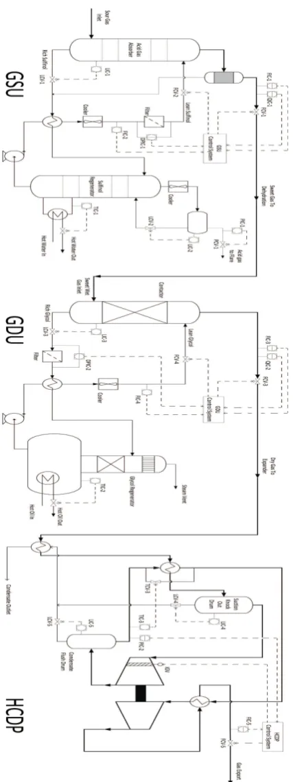
The process model of the gas train as sketched in Fig. 1 consists of three main processes; Gas Sweetening Unit (GSU), Gas dehydration Unit (GDU) and Hydrocarbon Dew-pointing (HCDP). Process models for each process in the gas train were developed in (Al-Naumani et al. (2016)). The models are based on a plant with a natural gas

specifi-cation of around 100bargpressure, 45℃ gas temperature

and a throughput flow rate up to 3.0MMSCMD(Million

Fig. 1. Gas Processing Train

described as high interaction control loops, presuming most other control loops are sufficiently controlled by SISO PID controllers.

2.1 GSU Model

Referring to the GSU in Fig. 1, the GSU system has two variables that have to be controlled, these are: the

throughput gas flow measured by FIC-1 and the acid

concentration in the gas outlet measured by the process

analyser QIC-1. The manipulated variables are: the

ab-sorber gas outlet flow through FCV-1 and the absorber

sulfinol input flow through FCV-2. The dynamics of the

GSU system are represented by the following 2x2 model:

GGSU =



  

−13.5

18.6s+ 1e

−2s 16.7

23.5s+ 1e

−6s

7.3

9.5s+ 1e

−13s 20

15.4s+ 1e

−6s



  

(1)

2.2 GDU Model

The Gas Dehydration Unit is downstream of the sweet-ening process as shown in Fig. 1. The GDU system has two variables that have to be controlled, these are: the

throughput gas flow measured by FIC-3 and the water

load in the gas outlet measured by the process analyser QIC-2. The manipulated variables are: the contactor gas

outlet flow throughFCV-3 and the contactor lean glycol

input flow through FCV-4. The dynamics of the GSU

system are represented by the following 2x2 model:

GGDU=



  

−8

15s+ 1e

−3s 19

30.3s+ 1e

−7s

6.2

13.5s+ 1e

−13s 10

16.7s+ 1e

−7s



  

(2)

2.3 HCDP Model

Referring to the GSU in Fig. 1, the Turbo Expander has two variables to be controlled to maintain the product

quality, these are: unit pressure measured byPIC-2 which

is located at the gas outlet of the condensate flush drum

and the load demand on the unit measured by FIC-5.

The manipulated variables are: the re-compressor outlet

flow measured throughFCV-5 and the expander inlet flow

through IGV (Inlet Guide Vanes). The dynamics of the

Turbo Expander are represented by the following model:

GH CDP =



   

0.2e−s

2s2_{+ 4s+ 1}

1

2s+ 1

0.3e−0.5s

0.4s2_{+s+ 1}

−0.3e−1.3s

0.1s2_{+ 3s+ 1}



   

(3)

3. PROPOSED CONTROL SYSTEM

There are many control system structure proposals in the literature, and indeed already being used in practice, which are likely to be feasible for a greenfield project (new plants) but not necessarily for brownfield ones (old plants). The feasibility of retro-fitting a new control structure is influenced by factors like project cost, system simplicity, process safety, running cost, and anticipated gains com-pared with the existing control system. Forbes et al. (2015)

concluded that Many industries do not necessarily need

better algorithms, but rather improved usability of exist-ing technologies to allow a limited workforce of varyexist-ing expertises to easily commission, use and maintain these valued applications.Critically, from an operational stand-point, the feasible control solution to enhance the current classical control system in existing oil and gas plants must

operational knowledge within it. Consequently, this section proposes a pragmatic alternative.

Al-Naumani and Rossiter (2015) provides the concept of the feasible solution by integrating small size MPC’s with the classical control system to handle the interactive con-trol loops in each process. The proposed concon-trol system, as in Fig. 2, integrates MPC as a master controller in the existing classical control of each subsystem. The MPC receives system measurements from the process sensors to compute the subsystem optimal control actions and pro-vide local control goals as set-points (SP) for the critical PID controllers only (high interaction control loops) while accounting for all process interactions. The MPC also receives system units status from the process safeguard-ing system to dynamically update the system constraints. However, a key point is that the MPC shares information like the next control move with its neighbour controllers to enhance the plant-wide optimal performance. This com-munication can help with disturbance rejection.

Fig. 2. Integration of MPC with classical control

The proposed control system is designed on a cascade strategy and thus provides a flexible system control almost like a decentralised structure in dealing with disturbances and unit failures, and at the same time improves the closed loop performance and the plant-wide optimal operation. The MPC is designed to regulate the critical loops only while the rest of the uncritical PID loops will continue to function in a decentralised fashion. This minimises any design and set up costs, reduces demand on the commu-nication network and simplifies any associated real time optimisations. The improved local control will reduce the need for control room operator interactions with their associated weaknesses. The one way communication from the process safeguarding enables prompt response to dis-turbances caused by unit failures while the bidirectional communications with adjacent MPC’s in effect enables feed-forward to reduce the impact of process disturbances and enhance optimality.

3.1 Challenges and Solutions of MIMO loops

Gas processing trains encompass three or more complex dynamic processes connected in series. These processes are coupled and contain a number of interactive control loops, although commonly controlled by conventional PID control laws. The potential drawback is that their perfor-mance and stability are sensitive to disturbances and load changes (Johansson et al. (1998)). Despite the vast array of PID tuning methods (Seborg et al. (2010); Romagnoli and Palazoglu (2012)), tuning MIMO PID controllers is still difficult and may not give good solutions (Johansson et al. (1998)). Poorly tuned interacting controllers severely limit

the best achievable closed loop performance and thus incur extra operational costs (Christofides et al. (2013)). On the other side, MPC has become a standard approach due to its ability to deal with process constraints and multi-variable systems (Forbes et al. (2015)). However, there are also drawbacks to the use of a single MPC to control, either an entire MIMO system in a centralised fashion or MIMO subsystems in a decentralised approach, which were thoroughly discussed by Al-Naumani and Rossiter (2015).

One obvious solution is to break up the control problem into subsystems and then separate SISO loops from the MIMO ones. SISO loops normally have no or low inter-actions with other loops and thus can be controlled by PID’s. Whereas the control of all MIMO loops in each subsystem will be indirectly allocated to a local MPC which in turn works as a master controller to regulate slave PID controllers that manipulate interactive control variables. Local MPC’s cooperate with the neighbouring system controllers by communicating their predicted

pro-cess outputs (y

→k

)n in order to account for interactions

between coupled processes.

3.2 Controllers Design and PID Controllers Setting

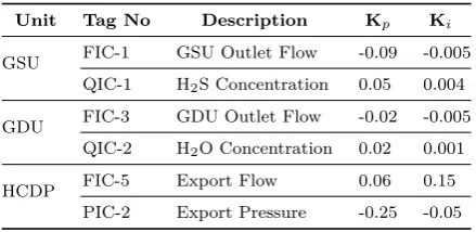
The control strategy of each subsystem incorporates: two SISO PID controllers in the inner control loops and one small MPC of dimension (2X2) in the outer loop. These PID controllers, categorised as critical PID’s, regulate the intermediate flow control valves between the subsystems. The settings are listed in Table 1.

Table 1. PID Controllers Settings

Unit Tag No Description Kp Ki

GSU FIC-1 GSU Outlet Flow -0.09 -0.005

QIC-1 H2S Concentration 0.05 0.004

GDU FIC-3 GDU Outlet Flow -0.02 -0.005

QIC-2 H2O Concentration 0.02 0.001

HCDP FIC-5 Export Flow 0.06 0.15

PIC-2 Export Pressure -0.25 -0.05

3.3 MPC Algorithm and Feed-forward

A matrix fraction description (MFD), representing the process of each subsystem with the relevant inner loop controls, were computed in order to construct the MPC law of the outer control loops. All MPC’s in Fig. 2 are multivariable Generalised Predictive Controllers (GPC) whose prediction is based on a MFD, thus take the form:

y →k+1

[i]_=H∆u

→k

[i]_{+P∆ u}

←k−1

[i]_+Qy

←k

[i]_+D[i]

n (4)

• y

→k+1

the vector of output predictions, ∆u

→kthe vector

of optimised input predictions, ∆ u

←k−1

is a vector of

past control increments and [i] represents the process

being controlled whether it is GSU, GDU, or HCDPU.

• H,P, andQare prediction matrices (e.g. see Rossiter

(2013)) and Dn is the feed forward term represents

Predicted process outputs, forwarded by predecessor

MPC’s, (y

→k

)nare continuously used to estimate the future

interaction between subsystems. Scaling factor matrices

(L) account for the severity of that process interaction on

the current system, hence: Dn =L[ i]

[(y

→k

)n− r

→] (5)

where r

→ is the future reference of the current process

as, typically, gas flow rates should match for each

pro-cess in the train. The scaling factor matrices (L) are

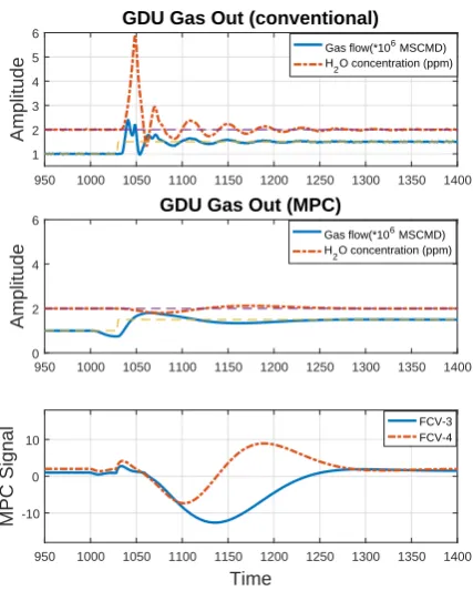
influenced by the strength of interactions between the relevant subsystems and can be computed by modelling the disturbance effects in the series processes. Gas quality of predecessor process does not influence the successor system behaviour but the gas flow rate does. Gas flow rate is the common controlled variable in all gas train processes. Fluctuations of the gas flow rate in a predecessor process has the potential to cause a sequence of disturbances in the successor processes. To demonstrate the effects, an almost 50% disturbance had been introduced to the GSU gas flow rate; and the effects on the successor processes gas flow rates are trended in Fig. 3. Gas train process disturbance

950 1000 1050 1100 1150 1200 1250 1300 1350 Time

0.8 1 1.2 1.4

Amplitude

GSU Gas flow(*106 MSCMD) GDU Gas flow(*106 MSCMD) HCDP Gas flow(*106 MSCMD)

X: 1026 Y: 1.475

X: 1088 Y: 1.388

X: 1078 Y: 1.094

Fig. 3. Process disturbance simulation of the gas train

simulation showed that, the disturbance in the GDU gas flow rate is about 82% of the GSU gas flow rate peak magnitude where the disturbance was generated. Whereas, HCDPU gas flow rate disturbed by about 25% of the GDU gas flow rate peak magnitude. The scaling factors are:

L[GDU]=

0.82 0

0 0

!

, and L[H CDP U]=

0.25 0

0 0

!

(6)

The GPC control law is then determined from a minimi-sation of a two norm measure of predicted performance:

min

∆u →

J =kr →−

y →

k22+λk∆u

→k

2

2 ₍₇₎

Consequently, the GPC control law is defined by the first

element of ∆uk =eT₁∆u

→

, eT

1 = [I,0,0, ...,0]:

∆uk=eT₁(HTH+λI)−1HT[r

→−

Py ←

−Q∆u ←−

Dn]

(8)

4. RESULTS

The proposed control structure was tested on the gas phase train model of Al-Naumani et al. (2016). The proposal was examined for two main causes of process disturbances; thus are sudden feed change and process unit malfunction.

4.1 Feed Disturbance

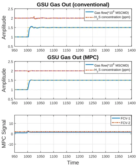
Process disturbances due to feed changes are common on upstream oil and gas plants and can be easily initiated by plant operators when changing process set points, or by an automated operation of process units. In practice, well tuned PID control system supported by experienced plant operators is capable of handling most of these disturbances to some extent. However, there are circumstances when the feed disturbances have the potential to cause a significant process upset due to the complex interactions of the underlying process. The disruptive nature of sudden feed changes is more of an issue for a series connected processes with MIMO loops. In order to compare the performance of the proposed control structure with the conventional one at a time of a sudden feed change, a 50% step up had been introduced to the gas flow setpoint of the GSU. The consequences on each process of the gas train are presented in Fig. 4 for GSU; Fig. 5 for GDU; and Fig. 6 for HCDPU. Process responses with conventional control system and the proposed control system were presented side by side for each process to aid comparisons between both systems.

950 1000 1050 1100 1150 1200 1250 1300 1350 1400 0.5

1 1.5 2 2.5

Amplitude

GSU Gas Out (conventional)

Gas flow(*106 MSCMD) H

2S concentration (ppm)

950 1000 1050 1100 1150 1200 1250 1300 1350 1400 0.5

1 1.5 2 2.5

Amplitude

GSU Gas Out (MPC)

Gas flow(*106 _MSCMD)

H

2S concentration (ppm)

950 1000 1050 1100 1150 1200 1250 1300 1350 1400

Time

-10 0 10

MPC Signal

FCV-1 FCV-2

Fig. 4. Comparison of GSU Process responses as a result of the 50% step increase in the (GSU) gas flow reference

950 1000 1050 1100 1150 1200 1250 1300 1350 1400 1

2 3 4 5 6

Amplitude

GDU Gas Out (conventional)

Gas flow(*106 MSCMD) H

2O concentration (ppm)

950 1000 1050 1100 1150 1200 1250 1300 1350 1400 0

2 4 6

Amplitude

GDU Gas Out (MPC)

Gas flow(*106 MSCMD) H

2O concentration (ppm)

950 1000 1050 1100 1150 1200 1250 1300 1350 1400

Time

-10 0 10

MPC Signal

FCV-3 FCV-4

Fig. 5. Comparison of GDU Process responses as a result of the 50% step increase in the (GSU) gas flow reference

950 1000 1050 1100 1150 1200 1250 1300 1350 1400 0

0.5 1 1.5 2

Amplitude

Export Gas Out (conventional)

Gas flow(*106 MSCMD) Pressure(*100 barg)

950 1000 1050 1100 1150 1200 1250 1300 1350 1400 0

0.5 1 1.5 2

Amplitude

Export Gas Out (MPC)

Gas flow(*106 MSCMD) Pressure(*100 barg)

950 1000 1050 1100 1150 1200 1250 1300 1350 1400

Time

-10 0 10

MPC Signal

FCV-5 IGV

Fig. 6. Comparison of HCDP Process responses following a 50% step increase in the (GSU) gas flow reference

4.2 Process Unit Malfunction

Process disturbances caused by a process malfunction or a sudden unit shut down are a major issue facing oil and gas companies. Practically speaking, the effects vary from a minor missed production targets to a total plant shut down depending on the criticality of the affected units on the process and the fault type. Process unit

malfunction is often an outcome of poor maintenance or harsh environment or simply a human mistake. To compare the performance of the proposed control structure with the conventional one at a time of a sudden process unit malfunction, a 10% sulfinol solvent filter chock had been introduced to the solvent control loop of the GSU. The result consequences on GSU, GDU, and HCDPU are presented sequentially in figures 7, 8, and 9 for both conventional and proposed control systems.

950 1000 1050 1100 1150 1200 1250 1300 1350 1400 0.5

1 1.5 2 2.5 3

Amplitude

GSU Gas Out (conventional)

Gas flow(*106 MSCMD) H

2S concentration (ppm)

950 1000 1050 1100 1150 1200 1250 1300 1350 1400 0.5

1 1.5 2 2.5 3

Amplitude

GSU Gas Out (MPC)

Gas flow(*106 MSCMD) H

2S concentration (ppm)

950 1000 1050 1100 1150 1200 1250 1300 1350 1400

Time

-10 0 10

MPC Signal

FCV-1 FCV-2

Fig. 7. Comparison of GSU Process responses as a result of the 10% solvent filter chock in the (GSU)

Once again, the MPC’s in the proposed control structure took prompt actions at the time of process disturbance to regulate slave PID controllers set points simultane-ously while accounting for all process interactions. GSU trends presented in Fig. 7 shows that, in the case of the

conventional control there are a sharp increase of H2S

concentration by nearly 40% of its initial reference value and spikes on the gas flow rate as a direct result of the solvent filter chock. Whereas the proposed solution shows a smooth control without spikes in both trends. The pro-posed control structure in both GDU Fig. 8, and HCDPU Fig. 9 shows a smooth and neat control trends, unlike the spiky trends in the conventional control case.

It is also noticeable from ‘MPC Signal’ trends in all units that, the processes are exclusively controlled by PID’s during stable operations; but at time of disturbances, MPC’s takes the lead and command corrective actions. This observation unveils a major advantage of the pro-posed control structure represented in the capability of the control system to remain functioning during MPC failure.

5. CONCLUSIONS

950 1000 1050 1100 1150 1200 1250 1300 1350 1400 0

1 2 3

Amplitude

GDU Gas Out (conventional)

Gas flow(*106 MSCMD) H

2O concentration (ppm)

950 1000 1050 1100 1150 1200 1250 1300 1350 1400 0

1 2 3

Amplitude

GDU Gas Out (MPC)

Gas flow(*106 MSCMD) H

2O concentration (ppm)

950 1000 1050 1100 1150 1200 1250 1300 1350 1400

Time

-10 0 10

MPC Signal

FCV-3 FCV-4

Fig. 8. Comparison of GDU Process responses as a result of the 10% solvent filter chock in the (GSU)

950 1000 1050 1100 1150 1200 1250 1300 1350 1400 0.5

1 1.5

Amplitude

Export Gas Out (conventional)

Gas flow(*106 _MSCMD)

Pressure(*100 barg)

950 1000 1050 1100 1150 1200 1250 1300 1350 1400 0.5

1 1.5

Amplitude

Export Gas Out (MPC)

Gas flow(*106 _MSCMD)

Pressure(*100 barg)

950 1000 1050 1100 1150 1200 1250 1300 1350 1400

Time

-10 0 10

MPC Signal

FCV-5 IGV

Fig. 9. Comparison of HCDPU Process responses as a result of the 10% solvent filter chock in the (GSU)

the disturbance influence in the process. As a result, the MPC actions improved the plant performance beyond what a skilled and experience operator can achieve. The results also prove the ability of the proposed control structure to reduce the disturbance effects in the series connected processes and to reduce the system dependency on operators. Splitting the MPC into smaller systems and dedicating it to control critical interactive loop only,

makes it easier to troubleshoot and to judge the behaviour of each MPC separately. But the biggest benefit of the proposed solution is that, all controlled variables will be under control even though one MPC is turned off for some reason (a set-up error for example).

Compared with the current solutions available in the literature (Negenborn and Maestre (2014)), the proposed control solution is cheaper because it builds up on the original plant control system structure. Also it is simpler to implement because the supervisory MPC control layer is small in size, furthermore it can be added to the existing control structure in the instrument auxiliary room without disturbing the field arrangements. The MPC system model is quite easy to develop for a small dimension problems, as well as the control algorithms. Nevertheless it almost delivers the same benefits and does not omit the team operational experience and maintenance skills. In addition it’s performance can be easily validated in the DCS by altering the cascade mode between auto and manual.

REFERENCES

Al-Naumani, Y. and Rossiter, J. (2015). Distributed mpc

for upstream oil & gas fields-a practical view.

IFAC-PapersOnLine, 48(8), 325–330.

Al-Naumani, Y., Rossiter, J., and Bahlawi, S. (2016). Gas phase train in upstream oil & gas fields: Part-i model

development. IFAC-PapersOnLine, 49(7), 875–881.

Bello, G. and Colombari, V. (1980). The human factors in risk analyses of process plants: The control room

operator model ‘teseo’. Reliability engineering, 1, 3–14.

Christofides, P.D., Scattolini, R., Mu˜noz de la Pe˜na, D.,

and Liu, J. (2013). Distributed model predictive con-trol: A tutorial review and future research directions. Computers & Chemical Engineering, 51, 21–41.

Forbes, M.G., Patwardhan, R.S., Hamadah, H., and

Gopaluni, R.B. (2015). Model predictive control

in industry: Challenges and opportunities.

IFAC-PapersOnLine, 48(8), 531–538.

Guerlain, S., Jamieson, G.A., Bullemer, P., and Blair, R. (2002). The mpc elucidator: A case study in the design

for human-automation interaction. IEEE Transactions

on Systems, Man, and Cybernetics-Part A: Systems and Humans, 32(1), 25–40.

Jipp, M., Moehlenbrink, C., Wies, M., and Lenz, H. (2011). Does cognitive lockup depend on the situation, on the

person, or on an interaction of both? In Proceedings

of the Human Factors and Ergonomics Society Annual Meeting, volume 55, 301–305. Sage Publications. Johansson, K.H., James, B., Bryant, G.F., and Astrom,

K.J. (1998). Multivariable controller tuning. In

Ameri-can Control Conference, 1998. Proceedings of the 1998, volume 6, 3514–3518. IEEE.

Negenborn, R. and Maestre, J. (2014). On 35 approaches

for distributed mpc made easy. In Distributed Model

Predictive Control Made Easy, 1–37. Springer.

Romagnoli, J.A. and Palazoglu, A. (2012).Introduction to

process control. CRC Press.

Rossiter, J.A. (2013). Model-based predictive control: a

practical approach. CRC press.

Seborg, D.E., Mellichamp, D.A., Edgar, T.F., and

Doyle III, F.J. (2010). Process dynamics and control.