R E S E A R C H
Open Access
Adaptive robust time-of-arrival source
localization algorithm based on variable step
size weighted block Newton method
Chee-Hyun Park
1and Joon-Hyuk Chang
2*Abstract
We propose a line-of-sight (LOS)/non-line-of-sight (NLOS) mixture source localization algorithms that utilize the weighted block Newton (WBN) and variable step size WBN (VSSWBN) method, in which the weighting matrix is determined in the form of the inverse of the squared error or as an exponential function with a negative exponent. The proposed WBN and VSSWBN algorithms converge in two iterations; thus, the required number of extra samples in the transient period is negligible. Also, we perform an analysis of the mean square error (MSE) of the weighted block Newton method. To verify the superiority of the proposed methods, the MSE performances are compared via extensive simulation.
Keywords: Block Newton method, Adaptive filter, Weighting matrix, Variable step size, Non-line-of-sight (NLOS)
1 Introduction
The aim of the source localization system is to find a geometrical point of intersection using the measure-ments from each receiver, such as the time difference of arrival (TDOA), time of arrival (TOA), or received sig-nal strength (RSS). Localizing a point source in which passive and stationary sensors are used has been a pop-ular research issue in the areas of radar, sonar, global positioning system, video conferencing, and telecommu-nication. Two key issues need to be resolved in source localization. The first is that the wireless localization sys-tems must be able to cope with rapidly varying channel conditions. To do this, adaptive filters have been impor-tant in adaptive source localization methods to stabilize localization performance under varying channel condi-tions [1–3]. However, these adaptive source localization algorithms were designed for the Gaussian noise situation and their localization performance is severely degraded in impulsive noise environments, such as Gaussian mix-ture and Student’s t distribution. Also, the convergence rate of the least mean square (LMS) algorithm adopted in
*Correspondence: [email protected]
2Department of Electronic Engineering, Hanyang University, Seoul 133-791,
Republic of Korea
Full list of author information is available at the end of the article
[1–3] may be much slower in some adverse environments. The second key issue is the challenge of localization in environments of line-of-sight (LOS)/non-line-of-sight (NLOS) mixture. LOS/NLOS mixture scenarios occur when there are obstructions between transmitters and receivers located in indoor environments and outdoor sit-uations such as urban areas. The localization performance of traditional approaches, which assume only LOS condi-tions, is severely degraded under NLOS conditions; thus, mitigation of NLOS errors has become an urgent task and has been extensively investigated in the last decade. In general, research of the LOS/NLOS mixture prob-lem for localization takes one of two approaches: (1) the constrained least squares (LS) method using optimiza-tion, such as semidefinite relaxation and second-order cone relaxation [4–9] and (2) localization based on the “NLOS identify and discard” [10–14]. Although localiza-tion using the optimizalocaliza-tion method has relatively high accuracy, the computational load is intensive. Localiza-tion using the “NLOS identify and discard” method also has relatively high accuracy when the LOS/NLOS mix-ture sensors are perfectly separated from the LOS sensors. However, the complete classification of LOS sensors and LOS/NLOS mixture sensors is nearly impossible, making it evident that classification error exists and the resulting
false classification incurs drastically increased localiza-tion error. Furthermore, when the number of sensors is large, the number of cases to be calculated is increased; thus, the computational burden is much high. Although our research results deal with the case in which the posi-tions of sensors are accurately known, some recent works assume the unknown coordinates of sensors [15–18].
The motivation for this paper is as follows. Adaptive localization methods have been proposed for position-ing in changposition-ing environments [1–3]. However, conven-tional adaptive localization algorithms, which minimize the squared error sum, are not robust to non-Gaussian noise (impulsive noise) situations, so they must be adapted to impulsive noise conditions. Our proposed algorithm minimizes the weighted squared error sum instead of the squared error sum, and the weighting matrix in the pro-posed algorithm counteracts the adverse effects of the LOS/NLOS mixture sensor. Namely, the weight is small when the sample is an outlier, which means an outlier-corrupted measurement is prevented from entering into the minimization of the cost function. Also, the conver-gence rate of the LMS method is slower than that of the Newton method and this slow convergence rate increases the number of samples in the transient period of the adap-tive filter and this is clearly a waste of resources. Thus, we propose a robust weighted block Newton (WBN) and variable step size WBN (VSSWBN) algorithms that use the Newton method instead of the LMS method. As can be seen from simulation results, the proposed WBN and VSSWBN methods converge in two iterations. Therefore, it is possible to neglect the number of additional sam-ples in the transient period of the adaptive localization algorithm.
The organization of this paper is as follows. Section 2 explains the LOS/NLOS mixture source localization prob-lem to be solved in this paper. In Section 3, the details of the existing localization methods are addressed. The pro-posed adaptive localization methods using the weighting matrix and variable step size are addressed in Section 4. The MSE analysis of the proposed WBN algorithm is per-formed in Section 5. The estimation performances of the proposed methods are evaluated via simulation results in Section 6, comparing them with those of the existing algo-rithms. Finally, the conclusion is presented in Section 7.
2 Problem formulation
The main goal of the TOA-based source localization method is to accurately determine the position of a source using multiple circles whose centers are the locations of sensors. In the LOS/NLOS mixture source localization context, the measurement equation is represented as
ri = di+ni=
(x−xi)2+(y−yi)2+ni, (1)
whereni∼(1−)N(0,σ12)+N(μ2,σ22),σ12σ22, i=
1, 2,. . .,M, with M denoting the number of sen-sors [7, 19–21]. Also,riis the measured distance between
the source and the ith sensor and di is the range
(dis-tance) model between the source and theith sensor. The measurement noiseni is modeled as a Gaussian mixture
distribution, where the LOS noise is distributed accord-ing toN0,σ12with a probability (1−) and the NLOS noise distributed byNμ2,σ22
with a probability of. It is assumed that while the statistics of the inlier can be obtained, the mean and variance of the outlier distribution are unknown. In practice,σ12can be estimated by observ-ing the energy bins in an absence of the transmitted signal and indeed the sample variance is usually adopted. Here, (0 ≤ ≤ 1) is the contamination ratio (i.e., fraction of contamination) which is a small number (typically smaller than 0.1) [7, 19–21]. Also, [x y]Tis the true source posi-tion and [xi yi]T is the position of theith sensor. Note
that, throughout this paper, a lowercase boldface letter denotes a vector, an uppercase boldface letter indicates a matrix and the superscriptT signifies the vector/matrix transpose. The purpose of this paper is to determine the source position that minimizes the MSE of the position estimate.
3 Review of the existing TOA localization methods
In this section, we briefly discuss the block LMS algo-rithm,M, and LMedS estimators in terms of the formula-tion of the source localizaformula-tion.
3.1 Block LMS source localization [1]
Squaring (1) and rearranging yield the following equation:
xix+yiy−0.5R+mi=0.5
(2) can be simply represented in a matrix form as
Ax+q=b, (3)
The block LMS location estimate is obtained iteratively as follows:
x(k+1)=x(k)+μATe(k) (4) wheree(k)=bk−Ax(k), superscript is the iteration
3.2 LMedS estimator
Classical LS regression consists of minimizing the sum of the squared residuals. In the LMedS algorithm, the sum is replaced by the median [22] of the squared residuals. The LMedS estimator can resist the effect of nearly 50% of the contamination in the data. The algorithm used to obtain a solution with this method can be summarized as follows [23]:
(1) Calculate them subsets of three measurements. (2) For each subsetS, compute a location by trilateration
PS.
(3) For each solutionPS, the residuesRSare obtained as
RS=
and the median of the residualsRSis computed.
(4) The solutionPS, which gives the minimum median, is determined as the source location.
3.3 M-estimator
The M-estimator is a class of robust estimator that has been considered for NLOS mitigation purposes. The loca-tion estimate using the M-estimator is obtained in the following: parameter to be estimated, andbiis the sample in theith
sensor. The standard deviation in (6) is an unknown value, so it should be estimated. The median absolute deviation (MAD), represented as s, is used as the estimate of the standard deviation and it is defined as
s=1.483 medi
where med is the abbreviation of the median. Also,ρ(·)is defined as follows:
ρ(ν)=
ν2/2 |ν| ≤η
η|ν| −η2/2 |ν|> η. (8)
Then, the position estimate using the M-estimator is obtained by using the Newton method as follows:
x(k+1)=x(k)+s(ATA)−1ATψ
and sign(·) is the sign function defined as sign(ν) = ⎧
4 Proposed adaptive robust localization methods In this paper, the LOS/NLOS mixture state is divided into the LOS and LOS/NLOS states. The LOS state denotes the case where the contamination ratio is zero (ε=0) and the LOS/NLOS state is the condition in which 0< ε≤1. The adaptive robust localization algorithms in this paper can be represented as follows.
4.1 WBN method
This proposed algorithm modifies the block LMS source localization algorithm [1] to robustify the block LMS algo-rithm against outliers by using a weighting matrix which is given as the inverse of the square error or an exponen-tial function with a negative exponent. Also, we adopt the block Newton method instead of the block LMS algorithm because the convergence rate of the Newton method is known to be much faster than that of the LMS algorithm [24]. The simulation results show that the MSE perfor-mance of the WBN algorithm converged in two iterations. The cost function to be minimized is defined as follows:
(b−Ax)TQ−1(b−Ax). (11)
The solution of the WBN method is represented as follows:
, ζ is a tuning parameter to be
deter-mined through offline work, e(k) = bk − Ax(k), bk =
b1,k· · ·bM,k
T
, andbi,kdenotes the sample of theith
sen-sor at thekth iteration. We use the weighting matrixQ(k)
to zero. In this case, the small positive value can be added to the squared residual for the stability of the algorithm.
4.2 WCBN method
The clipped LMS method has been widely used to reduce the complexity of the LMS algorithm [25]. The computa-tional complexity is reduced by clipping the input data to their polarity bits because the clipped LMS algorithm is a multiplication-free method. Following this algorithm, the matrixAis quantized by a sign function becauseAT in the block Newton method corresponds to the input signal in the conventional LMS algorithm. Then, the proposed WCBN algorithm is obtained as follows:
x(k+1) = x(k)+μ
The variable step size adaptive algorithm has been used to improve the MSE performance of the fixed step size adaptive method [26–28]. This algorithm updates the step size by minimizing the MSE cost function and adopting this technique to the WBN method yields the following iterative equation:
are generally selected through experiments to provide the maximum convergence rate preserving steady state mis-adjustment error small. The value ofμminis determined as
the level of steady-state misadjustment and the required tracking capabilities. The length of the transient period of the adaptive source localization method is desired to be short because the extra samples are consumed until the algorithm converges compared to the existing robust localization algorithm. Therefore, the step size is deter-mined as large as possible in the proposed method to aid fast convergence. In our simulation results, the VSSWBN algorithm showed a superior MSE performance and a sim-ilar convergence rate compared to the WBN method for large step sizes (both algorithms converged in two itera-tions). However, the MSE performances of the VSSWBN
and WBN algorithms were similar for small or medium step sizes.
5 Performance analysis
5.1 MSE performance analysis
This section presents the MSE analysis of the proposed algorithm. We derive the MSE of the WBN algorithm instead of the VSSWBN method for convenience of anal-ysis. The state error vector is represented as
x(k+1)−xo=x(k)−xo+μATQ(k)A−1ATQ(k)
wherexois the true source position. The steady-state error vector (v(∞)) can be attained as
where
and Q(l) was treated as the constant matrix for the ease of derivation. The WBN algorithm converges when
0 < μ < 1 from (18). In the derivation of the μ < 1. Note that the inverse of the squared error is rel-atively large in the LOS sensor and is small when the outliers exist. Then, althoughσ2is much larger thanσ1,
the MSE is nearly constant with respect to the standard deviation of NLOS noise and bias because the effect of large error standard deviation of LOS/NLOS mixture sen-sor inRlis attenuated by the weighting matrix Q(l) (see
(19) and (20)).
5.2 Computational complexity analysis
We compared the computational complexity for the local-ization algorithms. The computational complexities of localization methods are represented in the Table 1, and
M is the number of sensors, and N is the number of unknown variables to be estimated. The inverse and mul-tiplication operations for the matrix were mainly con-sidered because they are computationally intensive. The computational complexity of the VSSWBN method was higher than that of the WBN algorithm because it requires the additional computation of the step size. Also, the com-putational complexity of the WCBN method was lower than those of WBN and VSSWBN algorithms.
6 Simulation results
In this section, we compare the MSE performances of the proposed LOS/NLOS mixture source localization meth-ods with those of the M-estimator [22, 29] and LMedS estimator [23]. In these simulation settings, the source was assumed to be located within a 400-m2region to
deter-mine the performance over the entire area. Note that the
Table 1Comparison of the computational complexity
Algorithm Computational complexity
Block Newton OM2N
WBN O2M2N
VSSWBN O2M2N+M2
WCBN OM2
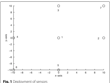
number of sensors used in this experiment was seven. Next, 30 different source locations were generated with a uniform distribution and sensors fixed. Five hundred Monte-Carlo simulations were performed for each given standard deviation of the NLOS noise. The standard devi-ation of the LOS noise of all of the sensors was assumed to be identical. In addition, the single and omni-directional source was assumed to be in the stationary state. The MSE average was calculated as follows:
MSE average= indicate theith true position of the source. Figure 1 illus-trates a deployment of sensors, in which the radius of the sensor network was set to 10 m. The localization accuracy as a function of the standard deviation of the NLOS noise is shown in Fig. 2. In Fig. 2a, the contamination ratio () was 20%, the standard deviation of the LOS noise (σ1) was
0.01 m, the bias of the NLOS noise (μ2) was 4 m, sensors
5, 6, and 7 were the LOS/NLOS sensors, and the remain-ing sensors were LOS sensors. The step size (μ) was set to 0.99 in the WBN algorithm. Also, the initial step size (μ(0)) was 0.99,ρwas 0.1, andμmaxandμminwere one and 0.01
in the VSSWBN algorithm. It is clear that the MSE aver-ages of the VSSWBN method are lower than those of other
−10 −8 −6 −4 −2 0 2 4 6 8 10
a
b
Fig. 2Comparison of MSE averages of the proposed estimators with those of the existing methods when the sensors 5, 6, and 7 are the LOS/NLOS mixture sensors and the remaining sensors are the LOS sensors.aContamination ratio (): 20%, the bias of NLOS noise (μ2): 4 m, standard deviation of LOS noise (σ1): 0.01 m.b: 30%,σ1: 0.01 m,μ2: 4 m
methods and nearly constant with respect to the stan-dard deviation of NLOS error. This observation is caused because the weighting matrix attenuates the effect of the large variance of LOS/NLOS mixture sensor. In Fig. 2b, the contamination ratio was 30% and the remaining condi-tions are the same as those in Fig. 2a. Figure 2b shows that the MSE average performances of the VSSWBN method are much superior to those of the other methods. Figure 3 assumes the same condition as that in Fig. 2, with the exception that sensors 4, 5, 6, and 7 are the LOS/NLOS sensors in Fig. 3. Again, the proposed VSSWBN method
3 4 5 6 7 8 9 10 −50
−40 −30 −20 −10 0 10 20
a
b
Standard Deviation of NLOS Noise (m)
MSE Average (dB)
WBN VSSWBN (19) Block Newton WCBN LMedS M Estimator
3 4 5 6 7 8 9 10 −50
−40 −30 −20 −10 0 10 20
Standard Devation of NLOS Noise (m)
MSE Average (dB)
WBN VSSWBN (19) Block Newton WCBN LMedS M Estimator
Fig. 3Comparison of MSE averages of the proposed estimators with those of the existing methods when the sensor 4, 5, 6 and 7 are the LOS/NLOS mixture sensors and the remaining sensors are the LOS sensors.aContamination ratio (): 20%, the bias of NLOS noise (μ2): 4 m, standard deviation of LOS noise (σ1): 0.01 m.b: 30%,σ1: 0.01 m,μ2: 4 m
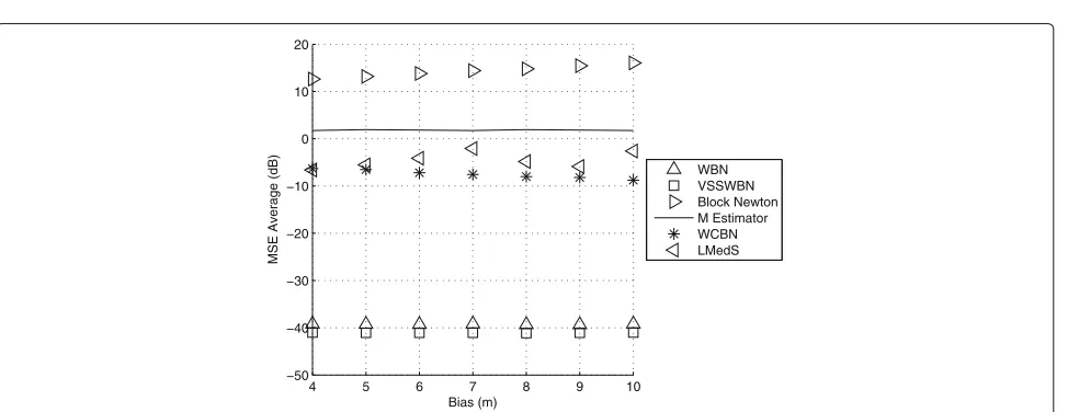
which attenuates the effect of large variance caused by the bias (μ22σ22 in (20)) because the corresponding weight is far small (squared residual is much large). Figure 7 shows the adaptation error as a function of the iteration num-ber when the impulsive noise exists in the 10th iteration. The WBN and VSSWBN methods converged in two iter-ations; thus, the additional samples which are required in the transient period are negligible. Additionally, the pro-posed WBN and VSSWBN algorithm accurately tracked the abrupt change caused by the impulsive noise. Figure 8 shows the MSE average of the proposed algorithms as a
0.1 0.2 0.3 0.4 0.5 0.6 0.7 0.8 −50
−40 −30 −20 −10 0 10 20
Contamination Ratio (ε)
MSE Average (dB)
WBN VSSWBN Block Newton WCBN LMedS M Estimator
Fig. 4MSE averages of the localization algorithms as a function of contamination ratio (bias of NLOS noise (μ2): 4 m, standard deviation of LOS noise (σ1): 0.01 m, standard deviation of NLOS noise (σ2): 10 m)
0 0.1 0.2 0.3 0.4 0.5 −50
−40 −30 −20 −10 0 10 20
Standard Deviation of LOS Noise (m)
MSE Average (dB)
WBN VSSWBN (19) Block Newton WCBN LMedS M Estimator
Fig. 5MSE averages of the localization algorithms as a function of standard deviation of LOS noise (bias of NLOS noise (μ2): 4 m, contamination ratio: 30%, standard deviation of NLOS noise (σ2): 10 m)
4 5 6 7 8 9 10
−50 −40 −30 −20 −10 0 10 20
Bias (m)
MSE Average (dB)
WBN VSSWBN Block Newton M Estimator WCBN LMedS
0 2 4 6 8 10 12 14 16 18 20 −20
−10 0 10 20 30 40 50
Iteration Number
Adaptation Error (dB)
WBN VSSWBN WCBN
Fig. 7Adaptation error of adaptive localization algorithms (contamination ratio: 30%, standard deviation of LOS noise (σ1): 0.01 m, standard deviation of NLOS noise (σ2): 10 m, bias (μ2): 4 m)
Fig. 8Comparison of MSE averages of the proposed estimators as a function of the number of sensors (when the number of LOS sensors increases)
5 6 7 8 9
−45 −44 −43 −42 −41 −40 −39 −38 −37
Number of Sensors
MSE Average (dB)
WBN VSSWBN
LOS/NLOS sensors is one when the number of sensors is five and then increases in parallel with the number of sen-sors. The MSE averages of the proposed methods decrease as the number of LOS/NLOS sensors increases, and the decreasing rate of the MSE averages is lower compared to the case in which the number of LOS sensors increases.
7 Conclusions
The WBN algorithm was developed by modifying the block LMS algorithm to make it robust to outliers and the proposed method employed a weighting matrix. Fur-thermore, the VSSWBN method was proposed to improve the MSE performances of the WBN algorithm. We also analyzed the MSE of the WBN algorithm. In the simula-tion results, the MSE averages of the proposed methods were smaller than that of the other adaptive localization methods and robust positioning algorithms.
Acknowledgements
This research was supported by Basic Science Research Program through the National Research Foundation of Korea (NRF) funded by the Ministry of Science, ICT, and Future Planning (No.2014R1A2A1A10049735).
Competing interests
The authors declare that they have no competing interests.
Authors’ contributions
In this research paper, the authors proposed a robust localization algorithm. All authors read and approved the final manuscript.
Publisher’s Note
Springer Nature remains neutral with regard to jurisdictional claims in published maps and institutional affiliations.
Author details
1Department of Electronics and Computer Engineering, Hanyang University,
Seoul 133-791, Republic of Korea.2Department of Electronic Engineering,
Hanyang University, Seoul 133-791, Republic of Korea.
Received: 22 February 2017 Accepted: 29 June 2017
References
1. CH Park, KS Hong, Block LMS-based source localization using range measurement. Digit. Signal Process.21(2), 367–374 (2011)
2. Y Sun, J Xiao, X Li, F Cabrera-Mora, inProc.of GLOBECOM. Adaptive source localization by a mobile robot using signal power gradient in sensor networks, (New Orleans, 2008), pp. 1–5
3. S Zhong, W Xia, Z He, inProc.of IEEE China Summit and International Conference on Signal and Information Process. Adaptive direct position determination of emitters based on time differences of arrival, (Beijing, 2013), pp. 230–234
4. S Venkatesh, RM Buehrer, inProc. of IEEE International Symposium on Information Processing in SensorNetworks (IPSN). A linear programming approach to NLOS error mitigation in sensor networks, (Nashville, 2006), pp. 301–308
5. X Wang, Z Wang, BO Dea, A TOA based location algorithm reducing the errors due to non-line-of-sight (NLOS) propagation. IEEE Trans. Veh. Technol.52(1), 112–116 (2003)
6. S Venkatesh, RM Buehrer, NLOS mitigation using linear programming in ultrawideband location-aware networks. IEEE Trans. Veh. Technol.56(5), 3182–3198 (2007)
7. Y Feng, C Fritsche, F Gustafsson, AM Zoubir, EM- and JMAP-ML based joint estimation algorithms for robust wireless geolocation in mixed LOS/NLOS environments. IEEE Trans. Signal Process.62(1), 168–182 (2014)
8. H Shen, Z Ding, S Dasgupta, C Zhao, Multiple source localization in wireless sensor networks based on time of arrival measurements. IEEE Trans. Signal Process.62(8), 1938–1949 (2014)
9. G Wang, H Chen, Y Li, N Ansari, NLOS error mitigation for TOA-based localization via convex relaxation. IEEE Trans. Wirel. Commun.13(8), 4119–4131 (2014)
10. YT Chan, WY Tsui, HC So, PC Ching, Time-of-arrival based localization under NLOS conditions. IEEE Trans. Veh. Technol.55(1), 17–24 (2006) 11. J Riba, A Urruela, inProc. of IEEE International Conference on Acoustics, Speech, and Signal Process. A non-line-of-sight mitigation technique based on ML-detection (ICASSP, Quebec, 2004), pp. 153–156 12. Y Qi, H Kobayashi, H Suda, Analysis of wireless geolocation in a
non-line-of-sight environment. IEEE Trans. Wirel. Commun.5(3), 672–681 (2006)
13. I Enosh, AJ Weiss, Outlier identification for TOA-based source localization in the presence of noise. Signal Process.102, 85–95 (2014)
14. A Abbasi, H Liu, Improved line-of-sight/non-line-of-sight classification methods for pulsed ultrawideband localisation. IET Commun.8(5), 680–688 (2014)
15. M Crocco, A Del Bue, V Murino, A bilinear approach to the position self-calibration of multiple sensors. IEEE Trans. Signal Process.60(2), 660–673 (2012)
16. I Dokmani´c, R Parhizkar, J Ranieri, M Vetterli, Euclidean distance matrices: Essential theory, algorithms and applications. IEEE Trans. Signal Process. Mag.32(6), 12–30 (2015)
17. T-K Le, N Ono, Closed-form and near closed-form solutions for TOA-based joint source and sensor localization. IEEE Trans. Signal Process.64(18), 4751–4766 (2016)
18. T-K Le, N Ono, Closed-form and near closed-form solutions for TDOA-based joint source and sensor localization. IEEE Trans. Signal Process.65(5), 1207–1221 (2017)
19. F Gustafsson, F Gunnarsson, Mobile positioning using wireless networks. IEEE Signal Process. Mag.22(4), 41–53 (2005)
20. U Hammes, E Wolsztynski, AM Zoubir, Robust tracking and geolocation for wireless networks in NLOS environments. IEEE J. Sel. Top. Signal Process.3(5), 889–901 (2009)
21. Y Feng, C Fritsche, F Gustafsson, AM Zoubir, TOA-based robust wireless geolocation and Cramer-Rao lower bound analysis in harsh LOS/NLOS environments. IEEE Trans. Signal Process.61(9), 2243–2255 (2013) 22. P Huber,Robust statistics. (Wiley, Hoboken, 2009)
23. R Casas, A Marco, JJ Guerrero, J Falco, Robust estimator for
non-line-of-sight error mitigation in indoor localization. EURASIP J. Adv. Signal Process.Article ID 43429, 1–8 (2006)
24. S Haykin,Adaptive filter theory. (Pearson, Upper Saddle River, 2013) 25. JL Moschner,Adaptive filtering with clipped input data.Ph.d.thesis.
(Stanford University, Stanford, 1970)
26. RH Kwong, EW Johnson, A variable step-size LMS algorithm. IEEE Signal Process.40(7), 1633–1642 (1992)
27. VJ Mathews, Z Xie, A stochastic gradient adaptive filter with gradient adaptive step size. IEEE Trans. Signal Process.41(6), 2075–2087 (1993) 28. B Farhang-Boroujeny,Adaptive filters: theory and applications. (Wiley,
Chichester, 2013)