Volume 2010, Article ID 323598,13pages doi:10.1155/2010/323598
Research Article
Introducing an Adaptive Method to Tune Initial Backoff
Window (CW
min
-ATM) in IEEE 802.11 Wireless Networks
Navid Tadayon and Saadan Zokaei
Electrical Engineering Department, Khajeh Nasir University of Technology, Tehran, Iran
Correspondence should be addressed to Navid Tadayon,[email protected]
Received 30 September 2009; Revised 29 December 2009; Accepted 14 March 2010
Academic Editor: Ping Wang
Copyright © 2010 N. Tadayon and S. Zokaei. This is an open access article distributed under the Creative Commons Attribution License, which permits unrestricted use, distribution, and reproduction in any medium, provided the original work is properly cited.
IEEE802.11 access protocol uses CSMA/CA in its Medium Access control layer as the main access function, which carries several deficiencies. In these networks, as the number of active stations increases, delay and throughput degrade severely. As far as throughput and service delay are vital elements in Quality of Service (QoS) determination, such degradation could lead to intolerable situations and reduce the efficiency of WLANs. Networks (WLANs). Studies proved this problem arises due to constant initial backoffwindows size (CWmin), which is an important parameter in determination of network behavior. In this paper, we
introduce a new method to tune this parameter adaptively according to changes in channel load. In this method, we do tune this parameter after every transmission using a feedback from transmission channel. Later it will be proven that applying this method in MAC layer enhances network stability; delay trend in all traffic classes exhibits a considerable reduction when compared with simple Enhanced Distributed Coordination Access (EDCA) scenarios. Also throughput exhibits a salient improvement in level. In other word, QoS improves. Especially, with the aid of this method, delay variations in all decrease considerably and more smoothen delay trends are achieved.
1. Introduction
In recent years, desires to utilize Local Area Network (LAN) for communication increased dramatically. Undoubtedly, one of the most important classes of these access networks
is IEEE 802.11 that was innovated in 1999 [1]. IEEE
802.11 networks work based on a contention-based access mechanism namely Carrier Sense Multiple Access supported with collision avoidance capability (CSMA/CA). This was the subject of investigation for many researchers during
these years [2–4]. As time went by and new, delay sensitive
services emerged with real-time requirements, attentions were attracted toward applying diff-serve model on IEEE 802.11 Medium Access control (MAC) layer. Henceforth,
many literatures focused on this subject [5–13].
Arrival of IEEE 802.11e standard into scene was a clear response to these efforts that have not been stopped yet.
In this paper, we follow the idea behind [14–16] which is
improving the 802.11 MAC performance using a channel
adaptive backoff scheme. We investigate the merits and
shortcomings of Distributed Coordination Function (DCF)
and Enhanced Distributed Coordination Access (EDCA) and verify their dependency on network parameters. It would be
claimed that using the legacy exponential backofftechnique
in DCF and EDCA leads to destructive dependence of
net-work performance on initial backoffwindows size, number
of stations, and network load. This is apparently a drawback from network viewpoint. By applying this adaptive method, each station could periodically estimate network load (by continuously hearing to channel activities). That helps us
directly in tuning of CWmin. Simulation results confirm the
suitability of this method.
We apply our proposed method on EDCA of IEEE 802.11e to probe its effect on different traffic classes. As DCF is a specific case of EDCA, the totality of argument is reserved.
2. Legacy IEEE 802.11
Data
NAV reset CTS
RTS Data Data Station defer
Data
ACK
Time (slot)
ACK ACK
Station deferred but 2 back offslot remains
Station set NAV upon receiving RTS
Station set NAV upon receiving CTS
Figure1: Interactions between six stations. In this example, station 6 is hidden from station 2 but can perceive station 1’s CTS.
2.1. DCF. The IEEE 802.11 MAC layer protocol is a dis-tributed coordination function and works based on carrier sense multiple access technique. In this technique, each station transmits its MAC service data units (MSDUs) after sensing the channel and ensuring that no transmission is in progress. In case two or more stations find channel idle and hence transmit simultaneously, the collision occurrence is inevitable. Therefore, IEEE 802.11 working group devised a mechanism, namely, collision avoidance, to reduce the collision probability. In this mechanism, stations start a
backoff procedure before transmission; to that end, they
should keep silent for a random amount of time imme-diately after channel remains idle for DCF Inter frame Space (DIFS). The DIFS value considered to be around
34μs in IEEE 802.11a standard. Upon the expiration of
this random time, stations are allowed to transmit. The length of this random time should be multiple of slot length. In fact, each station carries a parameter, namely, contention window from which this random time is to be extracted.
Upon the correct reception of each data frame, recipient terminal transmits an acknowledgement packet back to sender confirming the correct reception of previous data frame. In case a collision occurs, the contention window size is multiplied by a persistent factor (PF) mentioned in
standard. This mechanism is named exponential backoff. It
would be titled truncated exponential backoffscheme in case
there is an upper bound on contention windows size. All frames that would not be acknowledged during a predefined amount of time (ACK-Timeout) should be scheduled for retransmission; but with a doubled contention window size. This procedure definitely lessens the collision probability when several stations are attempting to access the channel.
Stations that deferred their channel access due to medium busyness, do not initiate a new random backoff time; instead, they continue to count down their most recent frozen values as soon as channel remains idle for at least DIFS. Finally, after each successfully transmitted MSDU,
a new random backoff procedure needs to be initiated
regardless of the fact that whether the transmitter queue is empty or containing an MSDU (ready to send). This routine
is entitled post backoffbecause of its initiation after each
transmission not before that.
Essentially, there is one case in which no backoff
procedure is required to be performed, that is, when, the
last post backoffhas already been finished while the queue
is still empty. Thus, an arrived MSDU from higher layer would be immediately transmitted without need to perform
a new backoffroutine. All other MSDUs coming after last one
should be transmitted after this backoffprocedure.
In order to reduce the collision length in long frames, the standard suggested fragmentation scheme. In this scheme, long MSDUs should be fragmented to a series of smaller units to be transmitted sequentially one by one and acknowl-edged as well. The principal benefit of fragmentation is that, in case of collision occurrence, errors are identified in a swifter manner. Apparently, fragmentation’s intrinsic drawback is the huge overhead it imposes on network.
In order to confront with hidden terminal problem, which is one of the most prevalent difficulties in CSMA/CA, Request to Send/Clear to Send (RTS/CTS) mechanism is devised. In this mechanism, sender station transmits a short control frame, namely, RTS prior to sending its data frame. Then, RTS recipient replies with another control frame, namely, CTS. Both RTS and CTS frames contain information about the length of following data frame. Following to reception of RTS by terminals in proximity of sender and reception of CTS by hidden terminals in proximity of receiver, all terminals should refrain from sending another frame in order to avoid collision occur-rence. In fact, this mechanism helps in protecting system against sending long collided frames, especially in situa-tions where hidden terminal problem is probable. Using Fragmentation, several smaller frames would be transmitted in series whereas using RTS/CTS method, a long frame would be transmitted but with less overhead and in a faster way.
In between each of RTS, CTS, Acknowledgment (ACK), and data transmissions, there should be idle separation intervals, namely, short inter frame space (SIFS) that is lower than DIFS, in length. Short Inter Frame Space (SIFS) value
is typically around 16μs (according to IEEE 802.11a
Defer access
Low priority TC
Medium priority TC
Higher priority TC
B-off
Count down as long as medium is idle, back-offwhen medium gets
busy again
Figure2: Comparison of different backoffclasses with different priorities.
SIFS’ length is always smaller than DIFS’ length, subsequent frames coming after SIFS intervals are logically furnished with relatively higher priority rather than frames coming after DIFS interval. Such an invention helps in providing ACK, RTS, and CTS with higher priority compared to Data frames.
3. Quality of Service Provisioning Mechanism in
802.11e Access Protocol
In order to support QoS in 802.11 wireless LANs, many proposals have been presented up to now and a lot more
are under studying. Recently, IEEE 802.11 task group E
approved a new standard by adding few enhancements to MAC layer of IEEE 802.11. The result is a new enhanced distribution coordination function, namely, EDCA. IEEE 802.11e constituted from two distinct access phases, namely, contention period (CP) phase and contention free period (CFP) phase. These two phases alternate steadily in a superframe framework over time. Like DCF, EDCA is a contention-based protocol that is utilized in CP phase.
3.1. EDCA. Now we commence with a definition of access category (AC). AC is the classification of different traffic classes in order to serve them with different requirements. To each AC in a station, a distinct EDCA is dedicated.
They perform backoffprocedure and act independently from
each other. Here, backoffprocedure starts immediately after
channel stays idle for AIFS duration. Depending on physical characteristic of each AC, Arbitration Inter Frame Space (AIFS) might extend from DIFS, which is the bottom value, to larger amounts. Immediately after waiting for AIFS, each
backoffentity sets its counter to an integer value extracted
uniformly from [1, CW + 1] interval where Contention Window (CW) in each AC varies from a minimum value,
namely, CWmin, up to the bound CWmax.
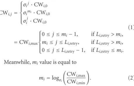
For traffic categoryi,let CWi,j denote contention
win-dow size at jthretransmission stage and let CWi,max denote
the maximum contention window size. Also,Li,retry,σi, and
miare, respectively, retry limit, persistent factor and number
of retransmissions after which CWi stays constant. (All in
class i.) Below equation encompasses all these parameters
and shows their interaction with each other.
CWi,j=
Meanwhile,mivalue is equal to
mi=logσi
Figure 2illustrates EDCA contention in different classes
with different priorities.
Figure 3is the Two-Dimensional Markov chain of
back-offmechanism in IEEE 802.11e networks.
Here, it just suffices to mention common equations of 802.11 and 802.11e networks without any proof. These equations are simply derivable from the discrete time Two-Dimensional Makov chain devised by Bianchi. We refer
inter-ested readers to [17, 18] for more details. Fundamentally,
the transmission probability in class i, is the probability
a given time slot (successful transmission or collision). We
express transmission probability byτi, collision probability
by pi, and busyness probability by pb. Below i, j, k,
respectively represent traffic category of that station (or
queue), retransmission stage, and value of backoffcounter
in each retransmission stage. Therefore,
bi,j,0=pij·bi,0,0, 0≤j≤Li,retry,
If we define the successful transmission probability as the situation in which at a given time slot all stations refrain
from transmission except one, then below equation would be apparent for this parameter:
ps,i=ni·τi·(1−τi)ni−1
In above set of equations,Mcorresponds to the number
of traffic categories exist in network andni to the number
of active stations surviving at classith. The absolute success
probability at a given station belonging to classi(instead of
conditional one computed above) is achieved after removing
the condition in (6) dividing it bypb. Hence,
Now we are ready to introduce two important quantities that will be exploited in our next section treatments; the first one is the mean number of station retries to transmit its packet successfully; the second one is the mean number of consecutive idle slots in an idle burst. These two quantities
play important roles in our treatments (referring to [18]):
Ns,i= 1
Up to now, we have presented formulas for EDCA. Hereafter, to the end of this section (and for the reason of simplification), we get back to DCF and extract a simplified equation for transmission probability based on absolute
collision probability,p. According to [17], the transmission
probability in DCF mode would be equal to
τ= 2·
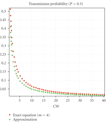
Figure 4 demonstrates that for larger m and smaller
p, the difference between two curves is trivial and the
approximation is well.
The larger the value ofm(the lower the value of p), the
better two curves fit each other.
1
Figure3: Two-Dimensional Markov chain of backoffmechanism in IEEE 802.11e networks.
immediately after DIFS idle time, whereas in EDCA the counter reduction is accomplished at the first edge of last AIFS idle slot. Although this little difference may not lead to a tangible influence on performance, it makes the analysis more convenient in EDCA case.
In EDCA mechanism, each station may have up to eight internal queues, each one representing a virtual station working independent of each other. In addition, each queue has its dedicated QoS parameters. When, two or more ACs (queue) inside a station attempt to transmit simultaneously, the virtual collision handler is activated. In this mechanism, among those ACs engaged in collision, the one with higher priority transmits right away and others refrain from trans-mission. This is in contrast with real collision situations in which two real concurrent transmissions lead to real
collisions.Figure 5illustrates this situation.
3.2. EDCA Performance Evaluation. In order to gain deeper understanding of our dynamic tuning scheme, we establish a set of simulations to study EDCA basic performance. The
aim of this section is to prove that differentiation mechanism
is only a tradeoff between different classes and cannot
improve the overall level of QoS in network. In other word, using differentiation methods, when one of QoS metrics (Throughput, Delay, Utilization...) improves in some classes, we should certainly expect to see degradation in other classes (on the same metric).
We utilized predefined model of IEEE 802.11e existing
in Opnet modeler.14 [19]. In this set of simulations, we
apply constant traffic load to a group of stations. Traffic is generated based on exponential interarrival rate and constant payload size, the condition that happens in many real situations. We set Mean interarrival time to 0.005 second and mean packet size to 1500 byte, what envisaged being a high load condition. In order to set up a stable working condition,
an offset time should elapse after simulation beginning
and before traffic generation in stations. To evaluate EDCA
performance, three traffic categories have been defined; first,
interactive multimedia class; second, interactive voice class;
third, Best effort class.
5 10 15 20 25 30 35 40
Transmission probability (P=0.3)
Figure4: Comparison of Exact and approximate Tau-CW plots. Evidently, the larger the value ofmis (the lower the value ofp), the better two curves fit each other.
Table1: Physical Layer Parameters.
Physical characteristic DSSS
Data Rate 5.5 Mbit/s
Transmit Power (W) 0.005
Packet Reception Power Threshold (dBm) −95
RTS Threshold (byte) None
Fragmentation Threshold (byte) None
CTS to Self Option Enabled
Short Retry Limit 7
Long Retry Limit 4
Max Receiver Lifetime (s) 0.5
Buffer Size (bits) 256,000
Roaming Capability Disabled
the only source of error is collision. Also hidden terminal possibility is avoided by putting all stations in hearing range of each other. For the sake of comparison, all three ACs benefit from the same traffic load condition. Other physical
layer parameters are cited atTable 1.
It is important to note that, no access point functionality is considered in this article and all stations work in a
distributed arrangement as illustrated inFigure 6.
Note that stations in each class only interact with each other, not with stations of other classes; that is to say voice by voice and video by video. At this section, we establish two sets of simulations; firstly, we evaluate network behavior by changing application load and secondly, we evaluate
performance by changing MAC layer parameters like CWmin,
Table2: MAC Layer Parameters.
AC CWmin(Slot) CWmax(Slot) AIFS (Slot) TXOP (μs)
VO 7 255 2 3264
VI 31 511 2 3264
BE 63 2047 2 3264
Transmission Opportunity (TXOP), and AIFS. In the first
set, we apply MAC parameters as mentioned inTable 2.
Figure 7 depicts load level and load variation for each of the tree scenarios. In each scenario, we have 100%
load increment than last scenario. Figure 8 depicts total
delay for these three different load conditions. This plot emphasizes that as stations’ load grows larger, delays increase boundlessly.
Figure 9 shows delay trends of voice class for three
different load situations (with 100% growth rate at each
situation). As other two classes exhibited the same trend as the voice class, we avoid showing them in this place.
Figures 10and11show, respectively, Delay-Time trend
and Delay-CDF (Cumulative Distribution Function) trend in all three classes under highest load condition (0.005 second). The comparisons simply reveal that higher priority class has greater chance to access the channel.
Now it is time to observe other parameters’ effects (like
CWmin, TXOP, and AIFS) on EDCA performance. Let us
start with CWmin. Firstly, we change CWmin in both voice
classes simultaneously and equally and observe its changing effects on delay value of all classes. As it is obvious, this changing should have direct influence on voice class delay as well as other class delays. However, the interesting fact is something else. The totals mean delay never changes in these scenarios; but what happens is just a simple tradeoff between classes meaning that higher priority class grasps more chance to transmit while the lower priority class looses it, and hence it starves; but the total mean stays always
intact. Figures12 and13are good illustrations to envisage
the situation. All parameter is the same as Table 2 but
the voice class CWmin that takes three values: 7, 31, and
63.
Because the best effort class showed the same trend
as video class, we avoid mentioning it here. By aggre-gating delays in all classes, we reach to below plot that discloses an important fact. The differentiation mechanism has no impact on overall delay improvement but instead is just a simple interclass tradeoff. This is evident from
Figure 14 that mean values are equal but depending on many factors we may decrease or increase delay variation (Jitter).
Now we have enough tools in hand to follow our aim, which is our novel adaptive tuning method.
4. Adaptive Method of Tuning Initial
Backoff Windows Size
B-off B-off B-off B-off B-off B-off B-off B-off B-off
Virtual collision resolver (grant TXOP to higher priority queue)
Transmission attempts Transmission attempts
AC AC AC AC AC AC AC AC AC
Higher priority Lower priority
802.11e EDCF 802.11 DCF
Figure5: ACs in each real station. There are eight traffic categories with different parameters in each station: (1) Left figure shown DCF with AIFS=34μs, CWmin=15, PF=2; (2) Right figure shown EDCA with AIFS [AC]≥34μs, CWmin[AC]=0–255.
12.5 25 37.5 50 62.5 75 87.5 100
75 62.5 50 37.5 25 12.5 0
Best effort 2
Video 1 Video 2
Voice 2 Voice 1
Objective
Figure6: Utilized topology. Six stations placed in equal distances in a Ring topology.
amount of successfully transmitted payload in a transmission period. Therefore,
Throu=Tpayload·psuccess
(Ts+NIdle)·pb.
(11)
This equation is logical and need no more explanation. In order to find an optimized point at which delay is minimized (and consequently throughput maximized), it is necessary
0 9.6 19.2 28.8 38.4 48 57.6 67.2 76.8 86.4 96 106 115 Interarrival time=0.005 s
Interarrival time=0.01 s Interarrival time=0.02 s 0
2 4 6 8 10 12 14 16
×106 WLAN load (bit/s)
Figure7: Load parameter depicted above for three scenarios. In each scenario, we have 100% load decrement than last scenario.
to find the maximal point of above equation by taking first derivative and equating it to zero. Therefore,
d(Throu)
d(CW) =0−→
d(Throu)
d(τ) ·
d(τ)
d(CW) =0,
d(τ)
d(CW)=/0 becauseτ=
2
CWmin·((1−P)/(1−2·P))+1.
0 7 14 22 29 36 43 50 58 65 72 79 86 94 101 108 115 Interarrival time=0.005 s
Interarrival time=0.01 s Interarrival time=0.02 s 0
0.1 0.2 0.3 0.4 0.5
0.6 WLAN total delay (sec)
Figure8: Total delay for each load condition. As load increases, the total delay grows correspondingly.
0 7 14 22 29 36 43 50 58 65 72 79 86 94 101 108 115
Interarrival time=0.005 s Interarrival time=0.01 s Interarrival time=0.02 s 0
0.02 0.04 0.06 0.08 0.1 0.12 0.14 0.16
0.18 WLAN voice class delay (sec)
Figure9: Voice class delay comparison for three load situations. As load increases, this quantity grows correspondingly.
This could be possible only ifd(Throu)/d(τ)=0. After
derivation and algebraic simplification:
(1−τ)n−2·(1−n·τ)·Ts−(Ts−1)·(1−τ)n
−n·(Ts−1)·τ·(1−τ)2·n−2
=0−→ Ts
Ts−1·(1−n·τ)
=(1−τ)n.
(13)
The intersection point atFigure 15represents the value
ofτat which Throughput maximized.
0 7 14 22 29 36 43 50 58 65 72 79 86 94 101 108 115 Best effort class
Video class Voice class
Interarrival time=0.005 s
0 1 2 3 4 5
6 WLAN delay of all classes (sec)
Figure10: Delay Time-Trend for all traffic classes (0.005-second interarrival time).
0.116 0.128 0.133 0.137 0.14 0.144 0.149 0.157 0.781 0.859 0.96 1.047 1.176 1.294 1.455 1.571 1.747 1.982 2.24 2.597 3.165 4.047 0
0.2 0.4 0.6 0.8 1 1.2
Best effort class Video class Voice class
Delay of all classes-CDF Interarrival time=0.005 s
Figure11: Delay CDF (Cumulative Distribution Function) Trend for all traffic classes (0.005-second interarrival time).
0
7.2 14.4 21.6 28.8 36 43.2 50.4 57.6 64.8 72 79.2 86.4 93.6 101 108 115
CWmin=7 slot CWmin=31 slot CWmin=63 slot 0
0.1 0.2 0.3 0.4 0.5 0.6
0.7 Voice class delay (sec)
0 9.6 19.2 28.8 38.4 48 57.6 67.2 76.8 86.4 96 106 115
2.5 Video class delay (sec)
Figure13: Video class delay decrease due to increment of voice class CWmin.
Time averaged total delay (sec)
Figure14: Altering voice class CWminhas no sensible impact on
Overall Delay although each class delay is affected differently.
0 0.2 0.4 0.6 0.8 1
Figure15: Optimum Tau value at which Throughput maximized (Intersection Point).
Backoffunit
Stage III
Last stage CWmin
Averaged and normalizedn(t)
Next stage CWmin
Figure16: Our proposed schematic flowchart diagram.
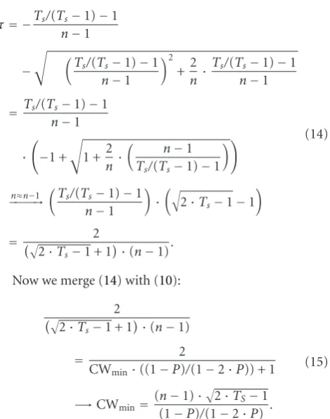
By further simplification in right hand side of equation, we reach to
τ= −Ts/(Ts−1)−1
Using this equation we could adaptively compute CWmin
as a function ofn(each terminal estimation of number of
contending stations is not the real number of stations!), p,
andTs. This equation constitutes the heart of our recycling
flowchart in third stage (Figure 16).
4.1. Schematic Diagram. To accomplish our task, we have drawn a schematic cyclic flowchart. Let us proceed through its all stages to derive appropriate practical equations. Up to
now, we have derived a suitable equation for third stage (14).
Now, its first stage’s turn!
4.1.1. Stage I. Let us suppose SB to be the number of busy slots observed by an observing station during a period of
busyness probability from this station’s perspective would be
using Newton’s equation, it turns possible to simplify above equation as
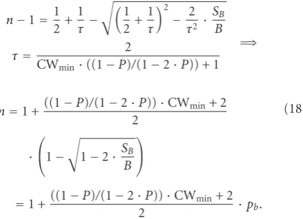
By further simplification of this equation and arranging
nas a function of CWmin andp and Coupling it with (10)
below equation is obtained:
n−1=1
This is a simple, linear, and effective equation and permits each station to estimate the number of contending terminal every time required. In cases of small busyness
probability, (light contention) √m
1−x≈1−x/mis a suitable
and tight approximation forx 1; thus, a linear equation
with least difficulty in computations is obtained. Aspb and
SB/Bare closely equal, we could apply them interchangeably.
4.1.2. Stage II. In order to avoid rapid and undesirable
changes in n(t), which arise from incorrect estimation of
pb or SB/B by stations, we devised an effective solution
with less error that could furnish network with larger stability and persistency. To that end, we utilize a buffer to
save several consecutive n(t) values. Then, by applying a
weighted normalization routine to these consecutive values, an implicit stabilizer is formed:
n(t+ 1)=α·n(t) + (1−α)
Clearly,αandqare both constant values that are tunable
depending on requirements. The larger α results in more
variable and instantaneousn(t+ 1) and hence an unreliable
behavior with greater variations, but with swifter acting
accomplished. Despite that, the smallerαvalue leads to stable
n(t+ 1) behavior with little variation and slow movements.
4.1.3. Stage III. At this stage we apply (15) to adaptively
compute CWminas a function ofn(t) (which is an estimation
of channel traffic). Finally, this initial window value will be exploited by stations for next transmissions.
4.1.4. Stage IV. As long asαvalue stays constant during
back-offperiods, we may expect trivial performance improvement
when working in adaptive tuning mode. To achieve better
improvements, it is better to tuneαat each stage according
to an appropriate logic. We have verified the fitness of below
set of equations (20) and a comparison done with a scenario
in whichαstayed static. The comparison proved a sensible
improvement in all quantities when dynamically tuning α.
For clarification, imagine below axis (Figure 17) that divided
into separate divisions by straight lines. Each part is a backoff period during which a packet will be transmitted successfully
after several trials. In addition,σt−jshows the mean variation
of CWminduringqlast periods. We are interested to findα(t)
for next period based on most recentα(namely,α(t−1)).
Thus, we follow these equations:
α(t)=α(t−1)·
As it is evident, our goal from exploiting several
summa-tions in this set of equasumma-tions is to have a smootherα(t) as far
as possible. The principal philosophy behind using the right
hand side equation is that, upon an abrupt change in CWmin
of previous stage, theα(t) increases automatically to provide
more dependency on exactly formern(t) rather than farther
ones (refer to equation. . . n(t+ 1)= · · ·).
Finally, when there was no variation in last stage of
CWmin,α(t) remains almost unchanged. We release further
0 7 14 22 29 36 43 50 58 65 72 79 86 94 101 108 115 Interarrival time=0.005 s
Adaptive tuning method Basic EDCF
0.9 WLAN delay (sec)
Figure 18: Total delay compared for both scenarios. Total delay
decreased in CWmin-ATM in comparison with EDCA.
0.23 0.26 0.28 0.29 0.31 0.32 0.32 0.34 0.36 0.38 0.39 0.41 0.42 0.44 0.46 0.48 0.49 0.53 0.58 0.63 0.68 0.73 0.78 0
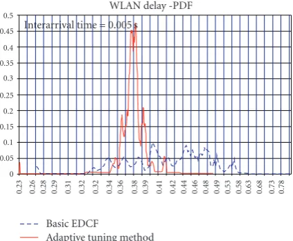
Adaptive tuning method WLAN delay -PDF Interarrival time=0.005 s
Figure19: Probability Density Function (PDF) of total delay for both scenarios. Jitter and Delay both decreased (Improved) in
CWmin-ATM.
5. Simulation Results
In this section, we present simulation results of adaptive tuning method proposed in last section. Again, all results are achieved by applying network parameters mentioned in
Tables1and2. In addition, all traffic generation parameters
are the same as what mentioned in Section 3.2 except
interarrival time that is set to be 0.005 s in these set of simulations.
We evaluated several performance measures like Delay (Media access delay), Jitter, Throughput, Retransmission Attempts, and utilization to support our claims as strong as possible. We compare our proposed scheme with common
EDCA in IEEE 802.11e. First, let us go over delay.Figure 18
shows the superiority of adaptive scheme against EDCA for total delay parameter.
0 7 14 22 29 36 43 50 58 65 72 79 86 94 101 108 115
Basic EDCF
Adaptive tuning method Interarrival time=0.005 s
0
0.4 Retransmission attepmts (packets)
Figure 20: Comparison of total retransmission attempts for
CWmin-ATM and basic EDCA method. Also this parameter lessened
considerably because collision probability is minor in CWmin-ATM.
Since Jitter (Delay Variation) is premier parameter in
telecommunication than absolute delay, Figure 19
demon-strates how in addition to gaining smaller delay, even smaller jitter is achieved in adaptive method. In fact, the narrower picked PDF is the evident to this claim.
Another important parameter is total retransmission attempt. It is the total number of retransmission attempts until either a packet is successfully transmitted or it is discarded (because of reaching short or long retry
limit).Figure 20shows this parameter lessened considerably
because collision probability is minor in adaptive method. Utilization is the measure of the consumption to date of available channel bandwidth. This quantity ranges between 0–100 where a value of 100.0 would indicate full usage.
Figure 21presents utilization improvement for three classes.
At last, Throughput results presented inFigure 22, which
is the total data traffic in bits/sec are successfully received
and forwarded to the higher layer by each access category of the WLAN MAC. Here, we only present total throughput
because we are interested to know how CWmin-ATM affect
overall system performance. This figure shows that total throughput increases in adaptive method. The underneath reason is the decreased collision probability that have direct influence on decreasing the number of packets dropped due to retry threshold exceeding and ones dropped due to overflow. Hence, throughput increases.
6. Conclusion
0 7 14 22 29 36 43 50 58 65 72 79 86 94 101 108 115 Interarrival time=0.005 s
Video class utilization (%)
70
100 Voice class utilization (%)
(b)
0 7 14 22 29 36 43 50 58 65 72 79 86 94 101 108 115 Best effort class utilization (%)
70
Adaptive tuning method Basic EDCF
(c)
Figure21: Utilization of Voice, Video, Best Effort classes for both
scheme (EDCA and CWmin-ATM). Video and best effort class
utilization improved (Lessened) but voice class utilization slightly increased.
The comparisons demonstrated that delay, throughput, retransmission attempt, and utilization were all positively
impacted when applying it in backoffprocedure of EDCA.
These are all network quantities that could be considered. The differences between results were far enough to decisively vote to suitability of this method.
In the coming paper, we proposed a new QoS improving method based on prioritization. We showed that it is possible
to combine CWmin-ATT and differentiation methods in
order to achieve better QoS in 802.11e networks.
0 10 19 29 38 48 58 67 77 86 96 106 115
Adaptive tuning method Basic EDCF
Interarrival time=0.005 s
Total throughput (bit/s)
Figure 22: Total throughput comparison for basic and adaptive methods. This figure shows that total throughput increases in adaptive method.
References
[1] “Wireless LAN Medium Access Control (MAC) and Physical Layer (PHY) Specifications,” IEEE standards 802.11, January 1997.
[2] M. S. Chhaya and S. Gupta, “Performance modeling of asynchronous data transfer methods of IEEE 802.11 MAC protocol,”Wireless Networks, vol. 3, no. 3, pp. 217–234, 1997. [3] A. Kumar, E. Altman, D. Miorandi, and M. Goyal, “New
insights from a fixed-point analysis of single cell IEEE 802.11
WLANs,”IEEE/ACM Transactions on Networking, vol. 15, no.
3, pp. 588–601, 2007.
[4] Y. C. Tay and K. C. Chua, “A capacity analysis for the IEEE 802.11 MAC protocol,”Wireless Networks, vol. 7, no. 2, pp. 159–171, 2001.
[5] J. Deng and R.-S. Chang, “A priority scheme for IEEE 802.11
DGF access method,”IEICE Transactions on Communications,
vol. E82-B, no. 1, pp. 96–102, 1999.
[6] Y. Xiao, “A simple and effective priority scheme for IEEE
802.11,”IEEE Communications Letters, vol. 7, no. 2, pp. 70–72, 2003.
[7] A. Veres, A. T. Campbell, M. Barry, and L.-H. Sun, “Sup-porting service differentiation in wireless packet networks using distributed control,”IEEE Journal on Selected Areas in Communications, vol. 19, no. 10, pp. 2081–2093, 2001. [8] I. Aad and C. Castelluccia, “Differentiation mechanisms for
IEEE 802.11,” in Proceedings of the 20th Annual Joint
Con-ference on the IEEE Computer and Communications Societies (INFOCOM ’01), vol. 1, pp. 209–218, Anchorage, Alaska, USA, April 2001.
[9] X. Pallot and L. E. Miller, “Implementing message priority policies over an 802.11 Based mobile ad hoc network,” in Pro-ceedings of Military Communications Conference (Milcom ’01), vol. 2, pp. 860–864, McLean, Va, USA, October 2001. [10] IEEE 802.11e WG, “Medium Access Control (MAC)
Enhance-ments for Quality of Service,” IEEE 802.11e/D2.0, November 2001.
[12] Y. Xiao, “IEEE 802.11 E: QoS provisioning at the MAC layer,”
IEEE Wireless Communications, vol. 11, no. 3, pp. 72–79, 2004. [13] Y. Xiao, H. Li, and S. Choi, “Protection and guarantee for
voice and video traffic in IEEE 802.11e wireless LANs,” in
Proceedings of the 23rd Annual Joint Conference of the IEEE Computer and Communications Societies (INFOCOM ’04), vol. 3, pp. 2152–2162, Hong Kong, March 2004.
[14] F. Cali, M. Conti, and E. Gregori, “IEEE 802.11 protocol:
design and performance evaluation of an adaptive backoff
mechanism,”IEEE Journal on Selected Areas in
Communica-tions, vol. 18, no. 9, pp. 1774–1786, 2000.
[15] J. Weinmiller, H. Woesner, J.-P. Ebert, and A. Wolisz,
“Mod-ified backoffalgorithms for DFWMAC’s distributed
coordi-nation function,” inProceedings of the 2nd ITG Fachtagung
Mobile Kommunikation, pp. 363–370, Neu-Ulm, Germany, September 1995.
[16] F. Cali, M. Conti, and E. Gregori, “Dynamic tuning of the IEEE 802.11 protocol to achieve a theoretical throughput limit,”
IEEE/ACM Transactions on Networking, vol. 8, no. 6, pp. 785– 799, 2000.
[17] G. Bianchi, “Performance analysis of the IEEE 802.11
dis-tributed coordination function,” IEEE Journal on Selected
Areas in Communications, vol. 18, no. 3, pp. 535–547, 2000. [18] E. Ziouva and T. Antonakopoulos, “CSMA/CA performance
under high traffic conditions: throughput and delay analysis,”
Computer Communications, vol. 25, no. 3, pp. 313–321, 2002.