A modified kernel method for a time fractional inverse diffusion problem

(1)

R E S E A R C H

Open Access

A modiﬁed kernel method for a

time-fractional inverse diffusion problem

Songshu Liu

1

_{and Lixin Feng}

2*

*_{Correspondence:}

[email protected]

2_{School of Mathematical Sciences,}

Heilongjiang University, Harbin, 150080, China

Full list of author information is available at the end of the article

Abstract

In this paper, we consider a time-fractional inverse diffusion problem, where the data is given atx= 1 and the solution is sought in the interval 0≤x< 1. Such a problem is obtained from the classical diffusion equation by replacing the first-order time derivative by the Caputo fractional derivative of order

α

∈(0, 1). We show that a time-fractional inverse diffusion problem is severely ill-posed and we further apply a modified kernel method to solve it based on the solution in the frequency domain. The corresponding convergence estimates are provided. Finally, an example is constructed to show the feasibility and efficiency of the proposed method.

MSC: 35R25; 35R30; 47A52

Keywords: time-fractional inverse diﬀusion problem; ill-posed problem; regularization method; error estimate

1 Introduction

In the past decades, studies on the problems of the partial differential equation mainly focused on direct problems and inverse problems of integer order differential equation, and some numerical techniques have been proposed to solve integer order differential equation [–]. However, fractional derivatives calculus and fractional differential equa-tions have been used recently to solve a range of problems in mechanical engineering [], viscoelasticity [], electron transport [], dissipation [], heat conduction [, ], and high-frequency financial data [].

The time-fractional diffusion equation arises by replacing the standard time partial derivative in the diffusion equation with a time-fractional partial derivative. It is usually used to describe the anomalous diffusion (superdiffusion, non-Gaussian diffusion, subdif-fusion) which is not consistent with the classical Fick (or Fourier) law []. The direct prob-lem,i.e., initial value problem and initial boundary for time-fractional diffusion equation have been studied extensively in the past few years [–]. However, in some practical problems, the boundary data on the whole boundary cannot be obtained. We only know the noisy data on a part of the boundary or at some interior points of the concerned do-main. This leads to an inverse and ill-posed problem of the fractional diffusion equation, which means the solution does not depend continuously on the given known conditions. In this paper, we investigate an inverse problem of the time-fractional diffusion equation. This kind of ill-posed problem is important in many branches of engineering sciences [, ].

(2)

Due to the difficulty of the fractional derivative and the ill-posedness, to the authors’ knowledge, the results on inverse problem of the time-fractional diffusion equation are very few. The uniqueness of an inverse problem for a one-dimensional fractional diffusion equation was given in []. Cheng and Fu [] gave an iteration regularization method for a time-fractional inverse diffusion problem. Zheng and Wei [, ] investigated a time-fractional inverse diffusion problem by using a spectral regularization method and a modified equation method.

In this article, we consider the following time-fractional inverse diﬀusion problem (TFIDP):

where the time-fractional derivativeDα

tu(x,t) is the Caputo fractional derivative of order

α∈(, ) deﬁned by []

where(·) is the gamma function.

The TFIDP is an inverse problem and is severely ill-posed. That means the solution does not depend continuously on the given data, and any small perturbation in the given data may cause large changes to the solution. In this paper, we will present a modiﬁed kernel method to construct a stable approximation solution of the TFIDP.

The rest of this paper is organized as follows. In Section , we demonstrate ill-posedness of the time-fractional inverse diﬀusion problem. In Section , a modiﬁed kernel method is used to solve problem (), and we also obtain the convergence estimates between the regularization solution and the exact solution based on thea prioriassumptions for the exact solution. In Section , an example is illustrated to show the main results. Finally, we conclude this paper in Section .

2 Ill-posedness of a time-fractional inverse diffusion problem

In order to apply the Fourier analysis of the time-fractional inverse diffusion problem, we extend all the functions to the whole line –∞<t<∞by defining them to be zero fort<  whenever it is necessary. We also assume all the functions involvingtvariable are inL₍_R_). Here, and in the following sections, we use the correspondingL_{norm, as defined below:}

(3)

be the Fourier transform of the functiong(t)∈L₍_R_{) and}_·

pdenote theHpnorm,i.e.,

gp=

∞

–∞

 +ξpg(ˆ ξ)dξ  

.

Then, applying the Fourier transforming with respect totto problem (), we have []

ˆ

ux(x,ξ) = –(iξ)αu(x,ˆ ξ), ()

ˆ

u(,ξ) =g(ˆ ξ). ()

The solution of the above problem can be given by

ˆ

u(x,ξ) =el(ξ)(–x)g(ˆ ξ), ()

where

l(ξ) = (iξ)α₌

⎧ ⎨ ⎩

|ξ|α₍_cosαπ

 +isin

απ

 ), ξ≥, |ξ|α₍_cosαπ

 –isin

απ

 ), ξ< .

For the above problem, note thatl(ξ) has a positive real part|ξ|αcosαπ

 , the small error in the high-frequency components will be ampliﬁed by the factore|ξ|αcosαπ_ (–x)_{. Therefore} the TFIDP for recovering the temperatureu(x,t) from the measured datagδ_{(t) is severely}

ill-posed. Here, suppose that the measured datagδ_(t)_∈_L₍_R_{) satisfy}

gδ_{(t) –}_g(t)_≤_δ_, _()

where the constantδ>  is the noise level.

To solve the problem (), a natural way to stabilize the problem is to eliminate the high frequencies or to replace the ‘kernel’el(ξ)(–x)_{by a bounded approximation.}

We now list two kernels of regularization methods for solving the time-fractional inverse diﬀusion problem.

The ﬁrst is

e(iξ)α_(–_x₎ χmax,

whereχmaxdenotes the characteristic function of interval [–ξmax,ξmax], andξmaxis a reg-ularization parameter. It corresponds to a spectral regreg-ularization method; see [].

The second is

e

(iξ)α +μξ(–x)_,

whereμis a regularization parameter. It corresponds to a modiﬁed equation method; see [].

In this article, we propose a regularization method by modifying the ‘kernel’ to deal with the diﬃculty of problem () as follows:

el(ξ)(–x)  +β_e|ξ|αcosαπ

 ,

(4)

Now, we will apply this regularization strategy to solve a time-fractional inverse diﬀusion problem and prove that this regularization strategy is feasible.

3 A modiﬁed kernel method and error estimates

In this section, we will construct regularization solution by modifying the ‘kernel’ and obtain convergence estimates.

Here, we give an approximate solution of problem () by perturbing the kernel of () as follows:

In order to obtain our main results, we ﬁrst give two important lemmas. Here, we set

η=|ξ|α_cosαπ

Combining () and (), we have

sup

Proof The proof of this lemma is similar to that of Lemma , we get the inequality ().

(5)

Theorem  Suppose that uβ,δ_(x,_t)_{is the regularization solution for problem}_()_{with noisy}

data gδ_(t)_{and that u(x,}_t)_{is the exact solution for problem}_()_{with the exact data g(t).}_Let

the assumptiongδ_{(t) –}_{g(t) ≤}_δ_{be satisﬁed and let}_u(,_{·) ≤}_{E hold.}_{If we choose}

β=δ

E, ()

then for every x∈(, ),we obtain the following error estimate:

uβ,δ(x,·) –u(x,·)≤δxE–x. ()

Proof By Parseval’s identity and the triangle inequality, we have

(6)

Therefore,

uβ,δ(x,·) –u(x,·)≤δβx–+Eβx,

according to (), we can get the error estimate

uβ,δ(x,·) –u(x,·)≤δxE–x.

The error estimate in Theorem  does not give any useful information on the continuous dependence of the solution atx= . To retain the continuous dependence of the solution atx= , one has to introduce a strongera prioriassumption.

We are now in the position to formulate the convergence rate forx= .

Theorem  Suppose that uβ,δ_(x,_t)_{is the regularization solution for problem}_()_{with noisy}

data gδ_(t)_{and that u(x,}_t)_{is the exact solution for problem}_()_{with the exact data g(t).}

Let the assumptiongδ_{(t) –}_g(t)_≤_δ_{be satisﬁed and let}_u(,_·₎

then,for x= ,we obtain the following error estimate:

uβ,δ_(,_·_{) –}_u(,_·₎

Proof It is similar to Theorem ; we obtain

(7)

and

The purpose of this section is to present a numerical example and illustrate the accuracy and eﬃciency of the proposed method. Here, the proposed methods will be implemented in Matlab. In our numerical experiment, we ﬁx the interval ≤t≤.

To illustrate the behavior of a modiﬁed kernel regularization method, we construct the test problems with a given functionf atx= , then we compute a data functiongatx=  according tog(ˆ ξ) =e–l(ξ)_fˆ₍_ξ_{), which is well-posed. We usually think that the computed} datag is exact. The discrete noisy datagδ _{is obtained by adding a random noise to the}

(8)

Then the total noiseδcan be measured in the sense of the root mean square error accord-ing to

δ:=gδ–g_l= 

n n

i=

gδ

i –gi

 .

Here, the functionrandn(·) generates arrays of random numbers whose elements are normally distributed with mean , varianceσ_{=  and standard deviation}_σ_{= , the} func-tionrandn(size(g)) returns an array of random entries that has the same size asg.

Example  Consider a smooth function

f(t) =

⎧ ⎨ ⎩

 t/e–



t, t> ,

, others.

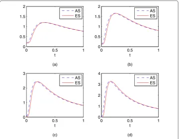
The comparison of the computational eﬀects withα= .,ε= ., atx= ., ., .,  are shown in Figure .

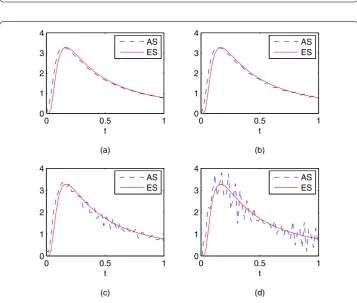
The comparison of the computational eﬀects withα= .,x= , forε= ., ., ., . are shown in Figure .

The comparison of the computational eﬀects withα= .,x= ,ε= . forγ = ., ., ., . are shown in Figure .

From Figures - (see also Tables -), we can ﬁnd that the numerical results near the boundaryx=  are better than the ones close tox= , and the smaller the parameterε,

Figure 1 The exact solution (ES) and its approximation solution (AS).α= 0.3,ε= 0.001 and(a)x= 0.8;

(9)

Figure 2 The exact solution (ES) and its approximation solution (AS).α= 0.4,x= 0 and(a)ε= 0.00001;

(b)ε= 0.0001;(c)ε= 0.001;(d)ε= 0.01.

Figure 3 The exact solution (ES) and its approximation solution (AS).α= 0.6,x= 0 and(a)γ= 0.6;

(10)

Table 1 The executing time for the running time program with differentxfor Example 1

x 0.8 0.5 0.2 0

t 9.420000 9.526000 9.483000 9.389000

Table 2 The executing time for the running time program with differentεfor Example 1

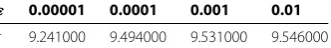
ε 0.00001 0.0001 0.001 0.01

t 9.241000 9.494000 9.531000 9.546000

Table 3 The executing time for the running time program with differentγ for Example 1

γ 0.6 0.7 0.8 0.9

t 9.346000 9.508000 9.514000 9.523000

the better the computed approximation is. Moreover, forx= , we can see that the smaller the parameterγ, the better the computed approximation is.

5 Conclusion

In this paper, we propose a modiﬁed kernel method for solving time-fractional inverse diﬀusion problem by producing a stable approximation solution. For this regularization strategy, in the presence of noisy data, we establish and prove the convergence estimates for the cases ≤x<  under thea prioribound assumptions for the exact solution and the suitable choices of the regularization parameter. From the results of numerical simu-lations, it seems clear that the proposed method works well for the model problem with small measurement error.

Competing interests

The authors declare that they have no competing interests.

Authors’ contributions

The authors contributed equally to the writing of this paper. All authors read and approved the ﬁnal manuscript.

Author details

1_{School of Mathematics and Statistics, Northeastern University at Qinhuangdao, Qinhuangdao, 066004, China.}2_{School of}

Mathematical Sciences, Heilongjiang University, Harbin, 150080, China.

Acknowledgements

This work was partially supported by National Natural Science Foundation of China (No. 11271113), the New Century Foundation of Heilongjiang Province (No. 1253-NECT-019) and Science and Technology Innovation Team in Higher Education Institutions of Heilongjiang Province (No. 2014TD005).

Received: 9 July 2015 Accepted: 26 October 2015 References

1. Arqub, OA, Al-Smadi, M: Numerical algorithm for solving two-point, second-order periodic boundary value problems for mixed integro-diﬀerential equations. Appl. Math. Comput.243, 911-922 (2014)

2. Arqub, OA, Al-Smadi, M, Momani, S, Hayat, T: Numerical solutions of fuzzy diﬀerential equations using reproducing kernel Hilbert space method. Soft Comput. (2015). doi:10.1007/s00500-015-1707-4

3. Arqub, OA, Al-Smadi, M, Shawagfeh, N: Solving Fredholm integro-diﬀerential equations using reproducing kernel Hilbert space method. Appl. Math. Comput.219, 8938-8948 (2013)

4. Arqub, OA, Abo-Hammour, Z: Numerical solution of systems of second-order boundary value problems using continuous genetic algorithm. Inf. Sci.279, 396-415 (2014)

5. Momani, S, Arqub, OA, Hayat, T, Al-Sulami, H: A computational method for solving periodic boundary value problems for integro-diﬀerential equations of Fredholm-Volterra type. Appl. Math. Comput.240, 229-239 (2014)

6. Alpay, D: Reproducing Kernel Spaces and Applications. Birkhäuser, Basel (2003)

7. Hon, YC, Wei, T: A fundamental solution method for inverse heat conduction problem. Eng. Anal. Bound. Elem.28, 489-495 (2004)

(11)

9. Chen, W, Ye, LJ, Sun, HG: Fractional diﬀusion equations by the Kansa method. Comput. Math. Appl.59, 1614-1620 (2010)

10. Yu, ZS, Lin, JZ: Numerical research on the coherent structure in the viscoelastic second-order mixing layers. Appl. Math. Mech.19, 717-723 (1998)

11. Scher, H, Montroll, EW: Anomalous transit-time dispersion in amorphous solids. Phys. Rev. B12, 2455-2477 (1975) 12. Szabo, TL, Wu, JR: A model for longitudinal and shear wave propagation in viscoelastic media. J. Acoust. Soc. Am.107,

2437-2446 (2000)

13. Gorenﬂo, R, Mainardi, F, Moretti, D, Pagnini, G, Paradisi, P: Discrete random walk models for space-time fractional diﬀusion. Chem. Phys.284, 521-541 (2002)

14. Metzler, R, Klafter, J: The random walk’s guide to anomalous diﬀusion: a fractional dynamics approach. Phys. Rep.339, 1-77 (2000)

15. Mendes, RV: A fractional calculus interpretation of the fractional volatility model. Nonlinear Dyn.55, 395-399 (2009) 16. Benson, DA, Wheatcraft, SW, Meerschaert, MM: The fractional-order governing equation of Lévy motion. Water

Resour. Res.36, 1413-1423 (2000)

17. Mainardi, F, Luchko, Y, Pagnini, G: The fundamental solution of the space-time fractional diﬀusion equation. Fract. Calc. Appl. Anal.4, 153-192 (2001)

18. Lin, YM, Xu, CJ: Finite diﬀerence/spectral approximations for the time-fractional diﬀusion equation. J. Comput. Phys.

225, 1533-1552 (2007)

19. Luchko, Y: Some uniqueness and existence results for the initial-boundary-value problems for the generalized time-fractional diﬀusion equation. Comput. Math. Appl.59, 1766-1772 (2010)

20. Mainardi, F, Pagnini, G: The Wright functions as solutions of the time-fractional diﬀusion equation. Appl. Math. Comput.141, 51-62 (2003)

21. Li, XJ, Xu, CJ: A space-time spectral method for the time fractional diﬀusion equation. SIAM J. Numer. Anal.47, 2108-2131 (2009)

22. Luchko, Y: Maximum principle for the generalized time-fractional diﬀusion equation. J. Math. Anal. Appl.351, 218-223 (2009)

23. Murio, DA: Stable numerical solution of a fractional-diﬀusion inverse heat conduction problem. Comput. Math. Appl.

53, 1492-1501 (2007)

24. Murio, DA: Time fractional IHCP with Caputo fractional derivatives. Comput. Math. Appl.56, 2371-2381 (2008) 25. Cheng, J, Nakagawa, J, Yamamoto, M, Yamazaki, T: Uniqueness in an inverse problem for one-dimensional fractional

diﬀusion equation. Inverse Probl.25, 115002 (2009)

26. Cheng, H, Fu, CL: An iteration regularization for a time-fractional inverse diﬀusion problem. Appl. Math. Model.36, 5642-5649 (2012)

27. Zheng, GH, Wei, T: Spectral regularization method for solving a time-fractional inverse diﬀusion problem. Appl. Math. Comput.218, 396-405 (2011)

28. Zheng, GH, Wei, T: A new regularization method for solving a time-fractional inverse diﬀusion problem. J. Math. Anal. Appl.378, 418-431 (2011)