Cell range expansion using distributed Q learning in heterogeneous networks

R E S E A R C H

Open Access

Cell range expansion using distributed

Q

-learning in heterogeneous networks

Toshihito Kudo

and Tomoaki Ohtsuki

Abstract

Cell range expansion (CRE) is a technique to expand a pico cell range virtually by adding a bias value to the pico received power, instead of increasing transmit power of pico base station (PBS), so that coverage, cell-edge throughput, and overall network throughput are improved. Many studies have focused on inter-cell interference coordination (ICIC) in CRE, because macro base station’s (MBS’s) strong transmit power harms the expanded region (ER) user equipments (UEs) that select PBSs by bias value. Optimal bias value that minimizes the number of outage UEs depends on several factors such as the dividing ratio of radio resources between MBSs and PBSs. In addition it varies from UE to another. Thus, most articles use the common bias value among all UEs determined by trial-and-error method. In this article, we propose a scheme to determine the bias value of each UE by usingQ-learning algorithm where each UE learns its bias value that minimizes the number of outage UEs from its past experience independently. Simulation results show that, compared to the scheme using optimal common bias value, the proposed scheme reduces the number of outage UEs and improves network throughput.

Introduction

Owing to the increase in demand in wireless bandwidth, serving by only macro base stations (MBSs) has become insufficient to serve the network’s user equipments (UEs). Subsequently, a recent solution, Heterogeneous networks (HetNets) whereby low power base stations (BSs) are deployed within the macro cell, has recently received significant attention in the literature [1]. HetNets are dis-cussed as one of the proposed solutions as part of the long term evolution-Advanced (LTE-Advanced) by the third generation partnership project (3GPP) [2].

As the low power BSs, some BSs are considered, for instance, pico BS (PBS), femto BS (FBS), relay BS, and so on. Among these low power BSs, PBSs are mostly con-sidered, because they can improve the capacity and they usually have the same backhaul as MBS. In [3], the authors place a PBS near the hot spot where the amount of traf-fic is high to prevent many UEs from accessing the MBS. PBSs have low transmission power, ranging from 23 to 30 dBm, and serve tens of UEs within a coverage range of up to 300 m [1]. However, in the presence of MBSs, PBSs’ ranges become smaller. MBSs’ transmit power is about 46 dBm, and the difference of them is about 16 dBm [1].

*Correspondence: [email protected]

Keio University, 3-14-1, Hiyoshi, Kohokuku, Yokohama, 223-8522, Japan

This big difference causes PBSs’ ranges to fall within tens of meters, whereas MBSs’ ranges are hundreds or thou-sands of meters [1]. This is not the case for uplink (UL), in which the reference signal strengths (RSSs) from a UE at different BSs mostly depend on the UE’s transmission powers [1]. Therefore, in this article, we consider only downlink (DL).

If the range of the hot spot area is the same as that of the pico cell, the PBS can serve UEs within that area and improve coverage area. However, because the hot spot’s location and amount of traffic change dynamically, PBSs cannot always cover the hot spot area and UEs may have to access the MBSs even if the PBS may be closer to them. In [1], the authors discuss cell range expansion (CRE), which is a technique that adds a bias value to pico received power from PBSs during the handover as if pico cell range is expanded, and many studies focus on this topic [1,3-9]. CRE can make more UEs to access the PBS even if the macro received power is stronger than the pico received power. However, those UEs that access the PBS whose pico received power is weaker than the macro received power are affected by a large amount of interference from MBS; such UEs are referred to as expanded region (ER) UEs [1]. Therefore, whenever CRE is used, inter-cell interfer-ence coordination (ICIC) may be needed so as to eliminate the interference.

Traditionally, UEs are set to use the same, fixed, bias value [1,3-8]. One reason is the fact that varying the bias value would require the measurement of the UEs’ distri-bution, which is hard to get. However, optimal bias values change depending on the location of UEs and BSs which differ from one another [4].

Owing to the difficulty to set the appropriate bias value for each UE, many articles mainly discuss applying ICIC[5-8]. ICIC is realized by dividing the radio resource: between two categories of MBS and PBS, ICIC is usually realized by stopping MBS’s transmission on some radio resources. ICIC is applied by separating frequency band in the frequency-domain approach instead of separating time slot in the domain approach. In the time-domain approach, almost blank subframe (ABS) [5] in which MBSs stop sending data and PBSs send to pico UEs (PUEs), particularly ER UEs, is mainly applied. However, even if ABS is used, reference signals are still transmit-ted by MBS, which causes interference [7]. To elimi-nate this interference, proposals in the literature include using lightly loaded controlling channel transmission sub-frame (LLCS) [7] or interference cancelation of common reference signal (CRS-IC) [8]. In the frequency-domain approach, furthermore, the restricted transmit power of MBS on the allocated frequency to PBS is also discussed in [9].

Resource blocks (RBs) introduced in 3GPP-LTE system [10] as blocks of subcarriers can also realize ICIC by divid-ing them between MBSs and PBSs [1]. Dependdivid-ing on this ratio of RB, the appropriate bias values also change, and this is also one reason for the difficulty to set optimal bias values. From these aforementioned reasons, optimal bias values are obtained only by using trial-and-error methods. Instead of using trial-and-error methods, we propose to useQ-learning [11], a machine learning (ML) technique, to determine the bias values. Using ML in radio com-munication system is becoming popular [12-17], because situations, where different radio systems are mixed in the same area, are very common, and since conditions change dynamically, adjustment of parameters is more difficult and complicated. Q-learning has been applied to many other areas such as cognitive radio [12] and inter-cell interference problem of multi-cell network [13]. It has also been applied to cellular networks, such as: self-organized and distributed interference management for femtocell networks [14], self-organized resource allocation scheme [15], cell selection scheme [16], and self-optimization of capacity and coverage scheme [17]. However, to the best of our knowledge, no studies applyQ-learning to setting the optimal bias value of CRE.

In this article, each UE learns the bias value that minimizes the number of outage UEs individually by Q-learning and can set the appropriate bias value inde-pendently. Simulation results show that, compared to the

trial-and-error approach to find the optimal common bias value, the proposed scheme reduces the number of outage UEs and improves average throughput in almost all cases.

Heterogeneous network

To solve coverage problems in MBS based homogeneous networks where only one BS serves UE in its coverage area, HetNets have been suggested in [18]. HetNets intro-duce remote radio head or low power BS such as PBS, FBS, and relay BS in a macro cell [1,18].

Though HetNets encompass many types of BSs, out of concern for simplicity, this work shall be limited to the case where only two types of BSs, namely MBS and PBS, as this is also the case in the majority of the related studies. PBSs are typically deployed within macro cells for capac-ity enhancement and coverage extension. Moreover, they usually have the same back-haul and access features as MBSs [1].

PBSs are deployed within macro cell to avoid having the hot spot UE access the MBS. Then, as the radius of a pico cell is limited, CRE [3] is traditionally used as we shall explain in the subsequent paragraph.

Cell range expansion

In this article, reference-signal-received-power-based (RSRP) handover [3], whereby the handover procedure is triggered through the assessment of the strength of the pilot signal (reference signal), shall be considered.

Using RSRP-based cell selection, UEs compare the power of reference signal from each BS, and connect to the largest one [3]. Moreover, using CRE, a bias value is added to the pico received signal, and more UEs can connect to PBSs, which is as if pico cell range is expanded. When UEs connect to MBS,

(wpilotm )dB> (wppilot)dB+(bias)dB. (1) When UEs connect to PBS,

(wpilotm )dB< (wppilot)dB+(bias)dB, (2) where (wpilotm )dB, (wpilotp )dB, and(bias)dB represent the decibel value of pilot signal power from MBS and PBS, and bias value, respectively, [1].

In this way, the pico cell range can be artificially extended. However, since ER UEs connect to BSs that do not provide the strongest received power, they suffer from interference from MBS [1].

The configuration of optimal bias value

Optimal bias values that minimize the number of outage UEs are changed by the ratio of radio resource among BSs and by the location of UEs and BSs. Since the optimal bias values vary from one UE to another [4], bias values should be defined by each UE. However, because of the difficulty to find the suitable sets of the ratio of radio resource and UEs’ distribution, most articles use the common bias value among all UEs [1,3]. In this article, each UE learns bias val-ues that minimize the number of outage UEs individually and can decide each bias value independently.

Reinforcement learning

Although supervised learning is effective, it may be hard to get training data on field. Thus, RL represents a suitable alternative as it only uses experiences of agents that learn automatically from the environment. In the RL, instead of the training data, agents get scalar values referred to as costs, and only these costs provide knowledge to agents [11].

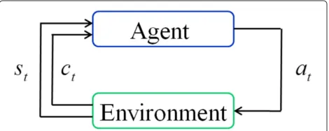
The interaction between the agents and their environ-ment, shown in Figure 1, can be summarized as follows:

1. Agents observe the statestof environment and make actionsatbased on the current observedstat the timet.

2. State transits to the next statest+1due to the execution of the selected actionat, and agents get costsctwhen executing actionatin statest. 3. Timet transits tot+1, then repeat steps 1 and 2. Thanks to the algorithm described above, RL is allowed an online learning which is one of the most important characteristic of RL.

Value function and policy

RL has two important components, policy and value func-tion.

Policy defines the action of agents at each step, in other words, policy is the mapping from observed state to an action that should be taken. It is expressed as a simple function, a look-up table, or other cases that need more exploration. Policy itself is enough to decide the action

Figure 1Interaction between agent and environment.

of agents [11]. It is represented as a probabilityπ(s,a)of selecting actionaat states. To calculate the policy means to decideπ(s,a)of all available actions at every state. The agent’s goal is to maximize the total amount of reward it receives over the long run.

Almost all reinforcement learning algorithms are based on estimating value functions—functions of states or of state-action pairs that estimate how good it is for the agent to be in a given state or how good it is to perform a given action in a given state. The expression of “how good” means the expected future rewards. Of course, the rewards that the agent can expect to receive in the future depend on what actions it will take. Accordingly, value functions are defined with respect to particular policies [11].

Recall that a policyπis a mapping from each statesand actionato the probabilityπ(s,a)of taking actionawhen in states. Informally, the value of a statesunder a policy π, denoted byVπ_{(s), is the expected return when starting}

where Eπ{·} denotes the expected value given that the agent follows policy π. Note that if the terminal state exists, its value is always zero. The functionVπ_{is referred} to as the state-value function for policyπ[11].

Similarly, the action-value function Q(s,a) can be defined, which is explained in the following subsection. In this article, action-value function Q(s,a) is used as the value function. This represents the value of select-ing action aat state s; this is theQ-value ofQ-learning explained later. The bestQ(s,a)denotes the best actiona at the states.

Q-learning

Q-learning is one of the typical methods of RL that is proved to converge in single agent systems [11,19]. Q-learning uses Q-value that means action-value func-tion. Agents have Q-table where they save the sets of states, actions, andQ-values that represent the effective-ness of the sets.

The goal of the agents is to minimize costs after select-ing actions. RL considers not only instant costs but also cumulative costs in the future that are represented as scalar value referred to asQ-value. It is defined as follows:

If the terminal state can be defined, costs are calculated up to the final one in Equation (4). However, since it can be rarely defined, the final time becomes infinity and future costs make Q-values diverse. That’s why a concept that discounting future costs is required. Ifγ = 0, agents do not care about future cost and consider only immediate costs, and ifγis about 1, agents have comprehensive views and consider the future costs.

It is very difficult to obtain optimal policy from Equation (4), because we cannot have the knowledge of all states. Therefore, instead of solving Equation (4), Q-learning is proposed in [11].

Equation (4) can be rewritten as follows [12]:

Q(s,a)=E{c(s,a)} +E mean value ofc(s,a), respectively. According to Equation (5), the current state’s Q-value can be evaluated by the current cost and the next state’sQ-value.

AllQ-values are stored per each state and action pair in Q-table and updated repetitively. Although because Q-learning has to save allQ-values, there may be a mem-ory problem, it can converge the action-value function Q(s,a) directly. Equation (4) can be approximately exe-cuted with using Q-table. It is enough to converge this learning if allQ-values of the sets of states and actions are continue to be updated. Because this concept is simple, it makes the analysis of algorithm easier.

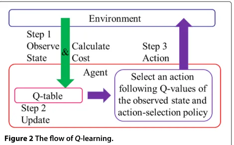
We describe the flow of Q-learning, illustrated in Figure 2, as follows.

Step (1) Agents observe their states from the environment and find the sets that have the state in theQ -table. They also get costs from the

environment as the evaluation of the selected actions. Step (2) Using the state and cost that are known at step (2), theQ -value selected at the previous state and action is updated.

Step (3) Following an action selection policy, for instanceε-greedy policy mentioned later, an action is selected making use of theQ -values of observed states at step (1).

Figure 2The flow ofQ-learning.

Through above steps,Q-learning realizes Equation (4). Q-value is updated as follows:

Q(st,at)←(1−α)Q(st,at)+α

whereαrepresents the learning rate (0< α≤1) that con-trols the amount of the change ofQ-value and “←” means update. This equation comes from Equation (5), and it considers future costs.

The aforementioned Q-learning algorithm has been

proved in the system of the single agent [19]. However, our system is the multi-agent system that has multiple agents, because all UEs can be the agents in our system. The con-vergence of Q-learning in a multi-agent system has not been proved in general, because of the complex relation-ship among the different agent. The multi-agent system has the proof of the convergence only when the agents do not move and know all the other agents’ strategies [20].

Cell range expansion withQ-learning

Though many articles use common bias value among all BSs and all UEs, UEs can improve coverage area by using their own bias values. Because of the difficulty to find the optimal bias value of each UE, in this article, we propose the scheme that every UE decides bias value indepen-dently to minimize the number of outage UEs by using Q-learning. Because all UEs should learn by themselves, in other words, all UEs can be the agents in our system, this system is a multi-agent system. Moreover, an online learn-ing which is allowed in the algorithm of RL is also used in our system.

areas. We show the example of such UE distribution in Figure 3. UEs and hot spots may move and hot spots’ moving speed is slower than UEs’ one.

We use RBs as radio resources and they denote blocks of subcarriers in this article. RB is the basic resource allocation unit for scheduling in 3rd-generation partner-ship project long term evolution (3GPP-LTE) system [10]. Although one or more RBs are considered to be allocated to UEs considered in 3GPP-LTE system [10], UEs can be allocated only one RB in this article. To eliminate the inter-ference from MBSs to ER UEs, RBs [1] should be divided into MBSs and PBSs. If UEs use the same RBs simulta-neously, there will be interference among the UEs. UEs, that do not get allocated RB by the BS, cannot access radio services.

Definition of state, action, and cost

We show the definition of state, action, and cost in Table 1.

• State:The state of timet is defined as:

st= {pM,pP} (7)

wherepMandpPdenote the received powers of the pilot signals from MBS and PBS, respectively. Although UEs can hear many signals from various BSs, they use the largest macro and pico ones, in other words, only two parameters are saved as state inQ -table. To make Q -table small, those two powers are quantized.

• Action:The action of timet is defined as:

at=b (8)

whereb denotes the bias value.

Figure 3UE’s distribution.+expresses UEs, red line means pico cell, and MBS is the center of this black circle. UEs move inside of this black circle. There is a hotspot around each PBS.

Table 1 The definition of state, action and cost

State pM: Received powers of the pilot signals from MBS.

pP: Received powers of the pilot signals from PBS.

UEs use the largest macro and pico ones.

Action b: The UE’s bias value

Cost n: The number of UEs that cannot get the radio service

because of no spectrum vacancy or weak received power, referred to as outage UEs.

Using the backhaul between BSs, we can calculate this number and broadcast it to UEs.

• cost:The cost of timet is defined as:

ct=n (9)

wheren denotes the number of UEs that cannot get the radio service because of no spectrum vacancy or weak received power, referred to as outage UEs. Using the backhaul between BSs, we can calculate this number and broadcast it to UEs.

On this definition, UEs decide bias values that min-imize the number of outage UEs depending on the received power from each BS. Furthermore, consider-ing the amount of radio resources, when there are many macro RBs (MRBs), access to the MBS may be better even if the difference is small, and vice versa. Each UE can cope with aforementioned situations and decide optimal bias value by usingQ-learning.

Flow of learning

We describe the flow of each UE’s learning as follows.

Step (1) Each UE receives pilot signals from each BS, and chooses the strongest macro and pico ones. In other words, each UE observes its state.

Step (2) The received power is quantized to converge faster, and each UE compares these pilot signal powers withQ -table’s states.

Step (3) If there are no equal received powers on each UE’sQ -table, they add new received powers to their ownQ -tables.

Step (4) Among those sets whose received powers are equal to the pilot signal powers, UEs usually choose one set that has the lowestQ -value or rarely choose one set randomly to avoid local minima asε-greedy policy [11].

Step (5) Each UE uses chosen set’s bias value as an action.

Step (6) Each UE compares “macro received power” with “pico received power” added by bias value, they try to connect to the larger one.

interfered by the MBS’s signals. Therefore, in this article, RBs are split.

Step (8) BSs calculate the number of outage UEs and pass it to UEs as a cost.

Step (9) Each UE reevaluates the chosen set’sQ -value at Step 4 as update based on Equation (6).

Step (1) to step (6) and step (9) are carried out by each UE, while step (7) and step (8) are done by BS.

Repeating the above steps makesQ-value of all sets of states and actions converge, and then agents can make right actions.

In our system, when the agents find a new state, if they always add them to theQ-table, the size ofQ-table increases, which is not allowed by the memory constraint. Moreover, this makes the learning time longer. To solve this, we use priori data of the common bias values to converge faster. The number of outage UEs of all the common bias values can be checked with trial-and-error method before starting to learn and sending data to make the learning time shorter, because the common bias val-ues are easier to know than the optimal bias valval-ues of each UE. Although the common bias values among all the UEs are not the best bias value for each UE [4], they are tend to be a close value to the best bias value of each UE. We also quantize received powers used as the state to be even values on step (2) and set upper and lower limits to check and remove outlier values. After outlier checking and quantization, state is added. By introduc-ing these, required memory size becomes smaller and the convergence becomes faster.

UEs keep having the data ofQ-table when they move to another PBS coverage area because even if the situation changes and if situations may have some similarities, the data got in one situations helps to learn in another situ-ation [21]. UEs use the data as the initial values of next learning, because we expect that it helps a learning algo-rithm to converge faster. Even in different situations, UEs learn environment so that the table is updated.

Simulation model and results

Each PBS has one hot spot, and hot spots are placed ran-domly around PBSs. A hot spot area has 25 UEs inside it and they are uniformly distributed. The rest 50 UEs are also uniformly distributed inside the macro cell. We show the simulation parameters in Table 2. Furthermore, in this simulation, as interval of bias value, we use 2 dB for Q-learning to makeQ-table small. The maximum value of bias value is 32 dB, in other words, the actions have 17 lev-els. As for states, however, agents in our scheme add new one toQ-table if they find it. Because of this characteristic, the number of states is not fixed. During the simulation, about 1600 states are observed.

Table 2 Simulation parameters [1,3]

Macro cell radius 289 m

Pico cell radius 40 m

Carrier Frequency 2.0 GHz

Bandwidth 10 MHz

RBs 50

Thermal noise density −174 dBm/Hz

Macro BSs 1

Pico BSs 2

Hot spots 2

UEs inside macro cell 50

UEs inside Hot spot areas 25

Macro BS transmit power 46 dBm

Pico BS transmit power 30 dBm

Macro path loss model 128.1+37.6 log₁₀(R)dB (R[km])

Pico path loss model 140.1+36.7 log₁₀(R)dB (R[km])

Velocity of UEs 3 km/h

Channel Rayleigh fading

trials 500000

Learning rate 0.5

Discount factor 0.5

ε 0.1

At first, we show the number of connected UEs and ER UEs when the ratio of RBs of PBS (PRBs), the splitting ratio between MBS and PBS is 40% that means the num-bers of RBs of pico and macro are 20 and 30, respectively (Figures 4 and 5). From Figure 4, we can see that the big-ger bias value, the larbig-ger the number of UEs that connect to PBS. This is because the number of ER UEs increases as bias value increases, as shown in Figure 5. However, a very large bias value reduces coverage area because it makes fewer UEs access to MBS and PBSs have fewer vacancies of RBs. From Figure 4, we can also see that the best bias value that connects most UEs to BSs exists. If we consider only the number of connected UEs, the bias value should be from 16 to 20 dB. Moreover, this optimal range of bias value is not fixed, because it depends on the location of UEs, hot spots, and BSs. We found that the bias values, that have the largest number of connected UEs, are not fixed, through the simulations.

Figure 4The number of connected UEs at each common bias value.The number of connected UEs at each common bias value. The ratio of PRB is 40%. No machine learning is used. MUE and PUE represent the UE that accesses MBS and PBS, respectively.

has low throughput, and it almost converges after about 50000 trials, and it has the best throughput after about 100000 trials.

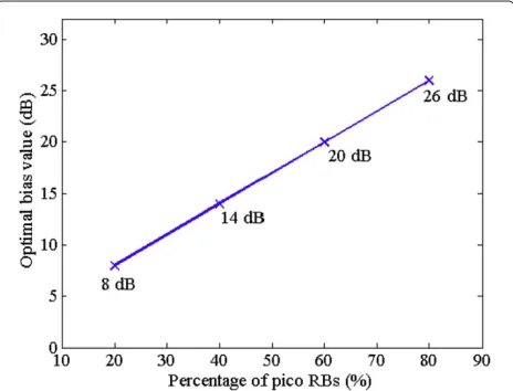
Figure 7 shows the bias values that have high probabil-ity to minimize the number of outage UEs. Optimal bias value that minimizes the number of outage UEs has linear increase as against the percentage of PRBs. This is because the higher a ratio of PRBs is, the more UEs can connect to PBS with controlling the bias value. Note that these values cannot always minimize the number of outage UEs.

From now on, we compare three schemes: the proposed Q-learning scheme, no learning scheme (best bias value),

Figure 5The number of ER UEs at each common bias value.The ratio of PRB is 40%. No machine learning is used.

Figure 6Convergence of average throughputs through trials.

The ratio of PRB is 40%. TheQ-learning scheme is compared with the schemes using fixed common bias values, 16 dB and 32 dB. To show the convergence, the throughput’s values are averaged per 10 trials.

and no learning scheme (fixed bias value). In the no learn-ing schemes, all UEs use a common bias value. Both no learning schemes use trial and error method and search the bias value that minimizes the number of outage UEs. No learning scheme (best bias value) searches the bias value that minimizes the number of outage UEs with trial and error method every time. Although it can get mini-mum number of outage UEs with using a common bias value, this is not practical because the best bias value can be found after checking the number of outage UEs of all bias values. Since the channel condition changes dynami-cally, they check these values at every trial, in other words,

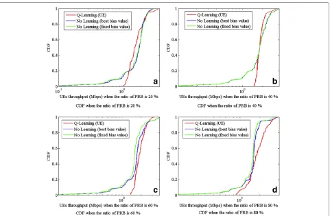
Figure 8CDF of UE throughputs.Average throughputs of all UEs through whole trials at the various ratios of PRBs. (a) CDF when the ratio of PRB is 20%. (b) CDF when the ratio of PRB is 40%. (c) CDF when the ratio of PRB is 60%. (d) CDF when the ratio of PRB is 80%.

this approach has the best performance in the case using common bias value. However, since it takes a bit long time to do that, it is not suitable in the real environment. Because of this, no learning scheme (fixed bias value) uses trial and error method only at the first trial as a practical scheme. These compared schemes use 1 dB as the inter-val of bias inter-value while 2 dB is used in our proposal. Note that the smaller interval results in better performance. In our proposal, to make the size ofQ-table small, a bit large interval, 2 dB, is used.

From Figure 8, we show the CDF of average through-puts of all UEs through all trials. Our proposal, the red line of Figure 8, can enhance the throughputs of the UEs who get weak received power such as cell-edge UEs. No learn-ing schemes have a lot of UEs who have weak received power while our proposedQ-learning scheme can serve high throughput to such cell-edge UEs. In spite of this fair-ness, when the ratio of PRB is 20%, the UEs of our proposal who are between about 0.2 and 0.7 of CDF in Figure 8a have lower throughputs than no learning schemes. When the ratio of PRB is 40 and 60%, the CDFs of our pro-posed scheme in Figure 8b,c are partially worse than no learning schemes. When the ratio of PRB is 80%, the CDF of our proposed scheme in Figure 8d are always better

than them. These results relate to the number of outage UEs and the UE’s average throughput in Figures 9 and 10 that are discussed below. No learning scheme (best bias value) can always be better than no learning scheme (fixed bias value).

Figure 9Average number of outage UEs at each ratio of RBs.

Figure 10Average throughput of all UEs at each ratio of RBs.

Q-learning approach compared to optimal common bias approach.

As shown in both Figures 9 and 10, the number of out-age UEs and the UE’s averout-age throughput change depend-ing on the ratio of PRBs. This is because bias values that minimizes the number of outage UEs also differ according to the ratio of RBs between MBS and PBS. The number of outage UEs changes depending on the ratio of PRBs. In spite of the rough interval,Q-learning, the red line of Figure 9, has fewer outage UEs than no learning schemes at almost all ratios of RBs. This means if UEs define their own bias values, we can get fewer outage UEs. When the ratio of PRBs is 20%, no learning schemes have fewer

outage UEs than Q-learning scheme. Many UEs have a

small difference between macro and pico received powers enough for the common bias value to occupy all RBs at this ratio. Of course, our proposal can also occupy all RBs at this ratio, however itsε-greedy policy’s occasional random actions make a bit more outage UEs. That is why no learn-ing schemes can keep the number of outage UEs smaller than that of the proposed scheme. In this figure, no learn-ing (best bias value) represents the minimum value of the number of outage UEs among the schemes using common bias value. Since the best bias value changes depending on some factors, no learning (fixed bias value) has more outage UEs than no learning (best bias value).

The same thing can also occur to the average through-put of all UEs in Figure 10. When the ratio of PRBs is 20%, no learning schemes have higher throughput than the pro-posed Q-learning scheme; except this ratio, Q-learning scheme performs better than no learning schemes.

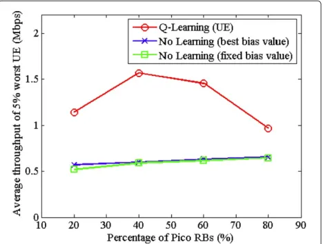
From the figures of CDF, we can confirm that our pro-posal can serve higher throughput to the UEs who get weak throughputs in the conventional scheme. Because in the 3GPP standard, cell-edge UE throughput is defined as 5% worst UE throughput [22], we also evaluate this value in Figure 11.Q-learning scheme has the best throughput

at all ratios of PRB. When the ratio of PRB is 40%, our pro-posed scheme has the largest improvement that is 61.7% higher than no learning scheme (best bias value). When the ratio of PRB is 20%, our proposal has worse average throughput of all UEs than no leaning schemes because of this enhancement of worst UE throughput. Although the common bias value among all UEs simplifies the con-trolling the system, cell-edge UE throughput degradation is revealed. This result shows that setting UE’s own bias value improves cell-edge UE throughput largely.

Conclusions

HetNets that introduce PBSs near hot spots in the macro cells are necessary to improve the coverage area. Since pico cell range may be too small to cover the hot spot area, pico’s CRE is considered. However, to the best of our knowledge, there have been no studies on the optimal bias value that minimizes the number of outage UEs, because this value depends on several factors such as the dividing ratio of radio resource between MBSs and PBSs, and it is determined only by trial-and-error method. Thus, in this article, we proposed a scheme usingQ-Learning that UEs learn bias values that minimize the number of outage UEs from past experience.

We got the results of the number of outage UEs and average throughput which show that after thousands of trials, the Q-learning approach can perform better than no learning schemes. We showed that our proposal can decrease the number of outage UEs and improve average throughput at almost all ratios of RBs. Moreover, it can largely enhance the cell-edge UE throughput compared with the schemes using a common bias value.

In the simulation, UEs keep having the data ofQ-table when they move to another PBS coverage area, and we

expect that it helps a learning algorithm to converge faster. However, we have not evaluated the effect of UEs’ mov-ing to other PBS coverage area in detail. This evaluation is our future study. The required learning time should also be studied for realizing this system because if it takes too much time to converge, it cannot be used in the real system.

Competing interests

The authors declare that they have no competing interests.

Received: 1 August 2012 Accepted: 4 February 2013 Published: 4 March 2013

References

1. D P´erez-L ´opez, X Chu, inProceedings of 20th International Conference on IEEE Computer Communications and Networks (ICCCN). Inter-cell interference coordination for expanded region picocells in heterogeneous networks, (Maui, HI, USA, 2011), pp. 1–6

2. A Damnjanovic, J Montojo, Y Wei, T Ji, T Luo, M Vajapeyam, T Yoo, O Song, D Malladi, A survey on 3GPP heterogeneous networks. IEEE Wirel. Commun.18, 10–21 (2011)

3. J Sangiamwong, Y Saito, N Miki, T Abe, S Nagata, Y Okumura, in11th European Wireless Conference 2011—Sustainable Wireless Technologies (European Wireless). Investigation on cell selection methods associated with inter-cell interference coordination in heterogeneous networks for LTE-advanced downlink, (Vienna, Austria, 2011), pp. 1–6

4. M Shirakabe, A Morimoto, N Miki, in8th International Symposium on Wireless Communication Systems (ISWCS). Performance evaluation of inter-cell interference coordination and cell range expansion in heterogeneous networks for LTE-advanced downlink, (Aachen, Germany, 2011), pp. 844–848

5. ˙I G ¨uvenc¸, MR Jeong, ˙I Demirdo ¯gen, B Kecicio ¯glu, F Watanabe, inIEEE Vehicular Technology Conference (VTC Fall). Range expansion and inter-cell interference coordination (ICIC) for picocell networks, (San Francisco, CA, USA, 2011), pp. 1–6

6. ˙I G ¨uvenc¸, Capacity and fairness analysis of heterogeneous networks with range expansion and interference coordination. IEEE Commun. Lett. 15, 1084–1087 (2011)

7. K Okino, T Nakayama, C Yamazaki, H Sato, Y Kusano, inIEEE International Conference on Communications Workshops (ICC). Pico cell range expansion with interference mitigation toward LTE-advanced heterogeneous networks, (Kyoto, Japan, 2011)

8. M Vajapeyam, A Damnjanovic, J Montojo, T Ji, Y Wei, D Malladi, inIEEE International Conference on Communications Workshops (ICC). Downlink FTP performance of heterogeneous networks for LTE-advanced, (Kyoto, Japan, 2011)

9. CS Chiu, CC Huang, inIEEE 75th Vehicular Technology Conference (VTC Spring). An interference coordination scheme for picocell range expansion in heterogeneous networks, (Yokohama, Japan, 2012), pp. 1–6 10. M Lee, SK Oh, in17th Asia-Pacific Conference Communications (APCC). On

resource block sharing in 3GPP-LTE system, (Sabah, Malaysia, 2011), pp. 38–42

11. RS Sutton, AG Barto,Reinforcement Learning(MIT Press, Cambridge, 1998) 12. A Galindo-Serrano, L Giupponi, DistributedQ-learning for aggregated

interference control in cognitive radio networks. IEEE Trans. Veh. Technol. 59, 1823–1834 (2010)

13. M Dirani, Z Altman, inProceedings of the 8th International Symposium on Modeling and Optimization in Mobile, Ad Hoc and Wireless Networks (WiOpt). A cooperative reinforcement learning approach for inter-cell interference coordination in OFDMA cellular networks, (Avignon, France, 2010), pp. 170–176

14. A Galindo-Serrano, L Giupponi, G Auer, inIEEE 73rd Vehicular Technology Conference (VTC Spring). Distributed learning in multiuser OFDMA femtocell networks, (Yokohama, Japan, 2011), pp. 1–6

15. A Feki, V Capdevielle, E Sorsy, inIEEE 75th Vehicular Technology Conference (VTC Spring). Self-organized resource allocation for LTE pico cells: a reinforcement learning approach, (Yokoham a, Japan, 2012), pp. 1–5

16. C Dhahri, T Ohtsuki, inIEEE 75th Vehicular Technology Conference (VTC Spring). Learning-based cell selection method for femtocell networks, (Yokohama, Japan, 2012), pp. 1–5

17. R Razavi, S Klein, H Claussen, inIEEE 21st International Symposium Personal Indoor and Mobile Radio Communications (PIMRC). Self-optimization of capacity and coverage in LTE networks using a fuzzy reinforcement learning approach, (Instanbul, Turkey, 2010), pp. 1865–1870 18. A Khandekar, N Bhushan, J Tingfang, V Vanghi, inEuropean Wireless

Conference (EW). LTE-advanced: heterogeneous networks, (Lucca, Italy, 2010), pp. 978–982

19. R Ribeiro, AP Borges, F Enembreck, inComputational Intelligence for Modelling, Control and Automation, International Conference. Interaction models for multiagent reinforcement learning, (Vienna, Austria, 2008), pp. 464–469

20. O Haitao, Z Weidong, Z Wenyuan, X Xiaoming, inProceedings of the 3rd World Congress Intelligent Control and Automation. A novel multi-agent

Q-learning algorithm in cooperative multi-agent system, (Hefei, China, 2000), pp. 272–276

21. A Galindo-Serrano, L Giupponi, P Blasco, M Dohler, inProceedings of the Fifth International Conference, Cognitive Radio Oriented Wireless Networks & Communications (CROWNCOM). Learning from experts in cognitive radio networks: the docitive paradigm, (Cannes, France, 2010), pp. 1–6 22. 3GPP TR 36.814 (V9.0.0), Evolved Universal Terrestrial Radio Access

(E-UTRA); further advancements for E-UTRA physical layer aspects (2010)

doi:10.1186/1687-1499-2013-61

Cite this article as:Kudo and Ohtsuki:Cell range expansion using dis-tributedQ-learning in heterogeneous networks.EURASIP Journal on Wireless Communications and Networking20132013:61.

Submit your manuscript to a

journal and benefi t from:

7Convenient online submission 7Rigorous peer review

7Immediate publication on acceptance 7Open access: articles freely available online 7High visibility within the fi eld

7Retaining the copyright to your article