Abstract
CICCO, TRACEY MARTINE WESTBROOK. Algorithms for Computing Restricted Root Sys-tems and Weyl Groups. (Under the direction of Dr. Aloysius Helminck.)
ALGORITHMS FOR COMPUTING RESTRICTED ROOT SYSTEMS AND
WEYL GROUPS
by
Tracey Martine Westbrook Cicco
a dissertation submitted to the graduate faculty of
north carolina state university
in partial fulfillment of the
requirements for the degree of
doctor of philosophy
mathematics
raleigh
March30,2006
approved by:
For Phil
Biography
Acknowledgments
I thank my family for so much: my best friend and husband Phil for his love, friendship, patience, and belief in me; my parents Oliver and Deborah for their unconditional support in letting me do it my way and for teaching me so much over the past twenty nine years; my sister Tanya and the Thorson family for showing me what else life has to offer.
Table of Contents
List of Tables xi
1 Introduction 1
2 Background 5
2.1 Root Data . . . 5
2.2 Actions on root data . . . 6
2.3 Restricted Roots . . . 7
2.4 Restricted fundamental system . . . 8
2.5 Restricted Weyl group . . . 9
2.6 Action ofGon∆ . . . 10
2.7 G-indices . . . 12
2.8 The index ofG . . . 13
2.9 Γ-index . . . 16
2.10 Notation . . . 17
2.11θ-index . . . 23
2.12 Root Space Decomposition . . . 24
3 The Algorithm 26 3.1 Step One: . . . 26
3.2 Step Two: . . . 26
3.3 Step Three: . . . 26
3.4 Step Four: . . . 27
3.5 Step Five: . . . 27
3.6 Step Six: . . . 27
4 Techniques used for Computing the Bases and Weyl Groups 28 4.1 A cases . . . 28
4.1.1 TypeA(1)n,n . . . 29
4.1.2 Type2A(1) 2n,n . . . 29
4.1.3 Type2A(1)2n−1,n . . . 29
4.1.5 TypeA(d)n,p . . . 30
4.1.6 Type2A(1)2n+1,n . . . 30
4.1.7 Type2A(1)n,p . . . 31
4.1.8 Type2A(d)n,p . . . 31
4.2 B case . . . 32
4.2.1 TypeBn,n . . . 32
4.2.2 TypeBn,n−1 . . . 32
4.2.3 TypeBn,p . . . 33
4.3 C cases . . . 33
4.3.1 TypeCn,n(1) . . . 33
4.3.2 TypeC2n,n(2) . . . 33
4.3.3 TypeC2n(2)+1,n . . . 34
4.3.4 TypeCn,p(2) . . . 34
4.4 D cases . . . 34
4.4.1 TypeD(1)n,n . . . 34
4.4.2 TypeDn,p(1) . . . 35
4.4.3 TypeD2n(2)+3,n . . . 35
4.4.4 TypeD2n,n(2) . . . 35
4.4.5 TypeDn,p(2) . . . 36
4.4.6 Type2D(1)n,n−1 . . . 36
4.4.7 Type2D(1) n,p . . . 36
4.4.8 Type2D(2)2n+2,n . . . 37
4.4.9 Type2D(2)2n+1,n . . . 37
4.4.10 Type3D(2)4,2 . . . 37
4.4.11 Type6D(2) 4,2 . . . 38
4.4.12 Type3D(9) 4,1 . . . 38
4.4.13 Type6D(9) 4,1 . . . 38
4.5 E6cases . . . 39
4.5.1 Type1E06,6 . . . 39
4.5.2 Type1E166,2 . . . 39
4.5.3 Type1E286,2 . . . 39
4.5.4 Type2E16 6,4 . . . 40
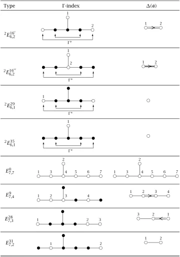
4.5.5 Type2E160 6,2 . . . 40
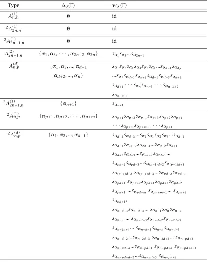
4.5.6 Type2E166,200 . . . 40
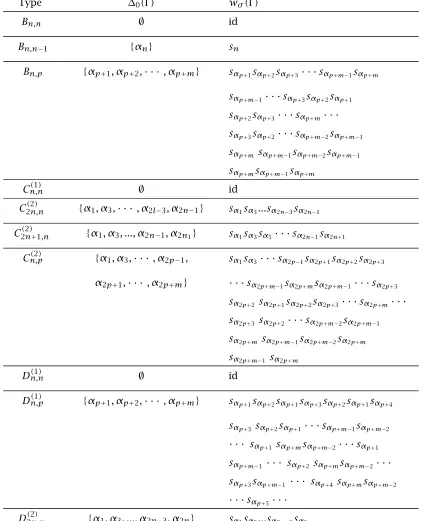
4.5.7 Type2E296,1 . . . 41
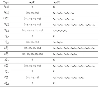
4.5.8 Type2E356,1 . . . 41
4.6 E7cases . . . 41
4.6.1 TypeE7,70 . . . 41
4.6.3 TypeE7,328 . . . 42
4.6.4 TypeE7,231 . . . 42
4.7 E8cases . . . 43
4.7.1 TypeE8,80 . . . 43
4.7.2 TypeE8,428 . . . 43
4.8 F4cases . . . 43
4.8.1 TypeF4,40 . . . 44
4.8.2 TypeF4,121 . . . 44
4.9 G2case . . . 44
4.9.1 TypeG02,2 . . . 44
5 Computing Weyl Group Elements 53 5.1 A cases . . . 53
5.1.1 TypeA(1)n,n . . . 53
5.1.2 Type2A(1) 2n,n . . . 53
5.1.3 Type2A(1)2n−1,n . . . 54
5.1.4 TypeA(2)2n+1,n . . . 54
5.1.5 TypeA(d)n,p . . . 54
5.1.6 Type2A(1) 2n+1,n . . . 54
5.1.7 Type2A(1)n,p . . . 55
5.1.8 Type2A(d) n,p . . . 55
5.2 B case . . . 55
5.2.1 TypeBn,n . . . 56
5.2.2 TypeBn,n−1 . . . 56
5.2.3 TypeBn,p . . . 56
5.3 C cases . . . 56
5.3.1 TypeCn,n(1) . . . 56
5.3.2 TypeC2n,n(2) . . . 56
5.3.3 TypeC2n(2)+1,n . . . 57
5.3.4 TypeCn,p(2) . . . 57
5.4 D cases . . . 57
5.4.1 TypeDn,n(1) . . . 57
5.4.2 TypeDn,p(1) . . . 57
5.4.3 TypeD2n(2)+3,n . . . 58
5.4.4 TypeD2n,n(2) . . . 58
5.4.5 TypeDn,p(2) . . . 58
5.4.6 Type2D(1)n+1,n . . . 58
5.4.7 Type2D(1)n,p . . . 59
5.4.8 Type2D(2) 2n+2,n . . . 59
5.4.10 Type3D(2)
4,2 . . . 59
5.4.11 Type6D(2) 4,2 . . . 60
5.4.12 Type3D(9)4,1 . . . 60
5.4.13 Type6D(9)4,1 . . . 60
5.5 E6cases . . . 60
5.5.1 Type1E06,6 . . . 60
5.5.2 Type1E16 6,2 . . . 61
5.5.3 Type1E28 6,2 . . . 61
5.5.4 Type2E16 6,4 . . . 61
5.5.5 Type2E166,20 . . . 62
5.5.6 Type2E166,200 . . . 62
5.5.7 Type2E296,1 . . . 62
5.5.8 Type2E356,1 . . . 62
5.6 E7cases . . . 63
5.6.1 TypeE7,70 . . . 63
5.6.2 TypeE7,49 . . . 63
5.6.3 TypeE7,328 . . . 63
5.6.4 TypeE7,231 . . . 64
5.7 E8cases . . . 64
5.7.1 TypeE8,80 . . . 64
5.7.2 TypeE8,428 . . . 64
5.8 F4cases . . . 64
5.8.1 TypeF4,40 . . . 65
5.8.2 TypeF4,121 . . . 65
5.9 G2case . . . 65
5.9.1 TypeG02,2 . . . 65
6 The Structure ofΦ(a)+ 70 6.1 A cases . . . 70
6.1.1 TypeA(1)n,n . . . 70
6.1.2 Type2A(1)2n,n . . . 71
6.1.3 Type2A(1)2n−1,n . . . 72
6.1.4 TypeA(2)2n+1,n . . . 74
6.1.5 TypeA(d)n,p . . . 74
6.1.6 Type2A(1)2n+1,n . . . 76
6.1.7 Type2A(1)n,p . . . 77
6.1.8 Type2A(d)n,p . . . 80
6.2 B cases . . . 85
6.2.1 TypeBn,n . . . 85
6.2.3 TypeBn,p . . . 87
6.3 C cases . . . 88
6.3.1 TypeCn,n(1) . . . 88
6.3.2 TypeC2n,n(2) . . . 88
6.3.3 TypeC2n(2)+1,n . . . 90
6.3.4 TypeCn,p(2) . . . 92
6.4 D cases . . . 96
6.4.1 TypeDn,n(1) . . . 96
6.4.2 TypeDn,p(1) . . . 96
6.4.3 TypeD2n(2)+3,n . . . 98
6.4.4 TypeD2n,n(2) . . . 103
6.4.5 TypeDn,p(2) . . . 105
6.4.6 Type2D(1)n+1,n . . . 108
6.4.7 Type2D(1) n,p . . . 110
6.4.8 Type2D(2)2n+2,n . . . 111
6.4.9 Type2D(2)2n+1,n . . . 114
6.4.10 Type3D(2)4,2 . . . 116
6.4.11 Type6D(2) 4,2 . . . 117
6.4.12 Type3D(9) 4,1 . . . 117
6.4.13 Type6D(9) 4,1 . . . 117
6.5 E6cases . . . 118
6.5.1 Type1E06,6 . . . 118
6.5.2 Type1E166,2 . . . 118
6.5.3 Type1E286,2 . . . 119
6.5.4 Type2E16 6,4 . . . 120
6.5.5 Type2E160 6,2 . . . 122
6.5.6 Type2E16"6,2 . . . 122
6.5.7 Type2E29 6,1 . . . 123
6.5.8 Type2E35 6,1 . . . 124
6.6 E7cases . . . 124
6.6.1 TypeE7,70 . . . 124
6.6.2 TypeE7,49 . . . 124
6.6.3 TypeE7,328 . . . 127
6.6.4 TypeE7,231 . . . 128
6.7 E8cases . . . 128
6.7.1 TypeE8,80 . . . 129
6.7.2 TypeE8,428 . . . 129
6.8 F4cases . . . 132
6.8.2 TypeF4,121 . . . 132
6.9 G2case . . . 133
6.9.1 TypeG02,2 . . . 133
7 An Example 134 7.1 Example2D(2) 8,3 . . . 134
7.1.1 Step 1: . . . 134
7.1.2 Step 2: . . . 134
7.1.3 Step 3: . . . 135
7.1.4 Step 4: . . . 135
7.1.5 Step 5: . . . 135
7.1.6 Step 6: . . . 136
7.1.7 Root Space Decomposition: . . . 137
List of Tables
2.1 Γ-indices . . . 18
4.1 wσ(Γ) . . . 45
4.2 Basis ofΦ(a)in terms of basis ofΦ(t). . . 48
Chapter 1
Introduction
In the last two decades computer algebra has had a major impact on many areas of math-ematics. Best known are its accomplishments in number theory, algebraic geometry and group theory. Several people have also started to devise and implement algorithms related to Lie theory. The most noteworthy examples of this are the packageLiEwritten by CAN (see [MLL92]) and the packages Coxeter and Weylby J. Stembridge, which are written in Maple (see [Ste92]). In theLiEpackage most of the basic combinatorial aspects of Lie theory have been implemented, following the excellent description and tables in [Bou81]. These mainly describe the fine structure of a root system with its Weyl group for a maximal torus of a reductive group defined over an algebraically closed field. (Or similarly of thek-split form of a group defined over a fieldk). There remain many, more complex aspects of Lie theory for which it would be useful to have a computer implementation of the structure. In this thesis we lay the foundation for a computer algebra package for computations related to all
k-forms of reductive groups defined over non algebraically closed fields. In the following we will callk-forms of these reductive groups:reductivek-groups.
with their Weyl groups and multiplicities of the roots plays a fundamental role in all studies of reductivek-groups and their applications.
In the case of reductive groups over algebraically closed fields the integrate fine structure related to the root systems with their Weyl groups has been implemented in several symbolic computation packages, like LiE, Maple, GAP4, Chevie, and Magma. These packages have become an indispensable tool for scientists in many areas of mathematics and physics. For reductive k-groups none of this fine structure has been implemented yet in a computer algebra package, although such a package would be extremely useful for many scientists as well. There are several reasons for this. The main reason is that the fine structure of these reductivek-groups a lot more complicated than that of the Lie groups, because instead of just 1 root system, there are 2 root systems which are closely entangled.
In this thesis we make the first step towards building a computer algebra package with which one can compute the fine structure of reductivek-groups.
All this fine structure of these reductivek-groups can also be computed in the Lie algebra setting, which simplifies some of the computations. To compute the fine structure of these reductive k-groups it does not suffice to compute the two root systems involved together with their Weyl groups. In many problems about these reductive k-groups one needs to know which roots project down to a root in a restricted root system and also one often needs representatives for elements of the Weyl group of the restricted root system in terms of representatives of the Weyl group of the related maximal torus. For example to compute nice bases for the root space decomposition of a reductive Lie algebra with respect to a maximalk-split torus one needs to decompose all root subspaces for roots of a maximalk -split toral subalgebraaas a sum of root subspaces of a maximal toral subalgebra containing
a. From theΓ-diagram corresponding to a reductivek-group (see section 2.9) one can easily determine this for the roots in a basis, but for all other roots we need the Weyl group and its action on the root subspaces of the maximal toral subalgebra to compute the decomposition of the root subspace of an arbitrary root of a. So computing the fine structure of these reductivek-groups will include computing representatives for the restricted Weyl groups in terms of Weyl group elements of the maximal toral subalgebra and also computing all the roots that project down to a root in a restricted root system.
by Tits in [Tit66]. Forg simple defined over a fieldk which is algebraically closed, the real numbers, thep-adic numbers, a finite field or a number field there are 45 different types of
Γ-indices which are absolutely irreducible. For each of these 45 types of Γ-indices we give an algorithm to compute their fine structure, which is roughly as follows. LetΦdenote the root system of the maximal toral subalgebra and∆= {α1, . . . , αn}a basis ofΦcompatible with theΓ-index.
(1) Using theΓ-index, determine the elements ofΓ.
(2) Find a basis ¯∆= {λ1, . . . , λr}of the restricted root system in terms of∆by finding the projection of eachαj in∆,and determine eachλiin terms ofαj.
(3) Note the type of restricted root system, and determine a representative wi in the Weyl group of the maximal toral subalgebra for each sλi, with λi ∈ ∆¯. This gives
representatives of the Weyl group of Φ(a) in the Weyl group of the maximal toral subalgebra.
(4) DetermineΦ(λi):= {α∈Φ|π (α)=λi}for eachλiin Step (1).
(5) Find the roots inΦ(a)+using the Weyl group as determined in step (3). (6) ComputeΦ(λ)for eachλ∈Φ(a)+by using the fact thatλ=w(λ
i)for somew ∈W (a),
λi∈∆¯and using the fact thatΦ(λ)=Φ(w(λi))=w˜Φ(λi), where ˜wis a representative ofw∈W (a)in the Weyl group of the maximal toral subalgebra and ˜w is a product of thewias above.
Note thatΦ(−λ)= −Φ(λ), so to determine the structure ofΦ(a), it suffices to determine
Φ(λ)forλ∈Φ(a)+.
The computation of this fine structure can be used to compute nice bases for the root space decomposition with respect to a maximalk-split toral subalgebra.
A brief summary of the contents follows. In chapter 2 we will lay the theoretical foun-dation for developing algorithms for a computer algebra package for the fine structure of reductive k-groups by proving a number of results about group actions on root data. We also show how these results can be used to compute the root space decomposition of a reductive Lie algebra with respect to a maximalk-split torus.
Chapter 3 outlines the six steps of the algorithm to be followed for each type ofΓ-index. In chapter 4, we determine the action ofΓ and compute the projection of eachαi for each type of Γ-index. This completes steps 1 and 2 of the algorithm. The results of these first two steps are included in tables at the end of chapter 4.
In chapter 5, we determine the Weyl group representative wi for eachsλi. The findings
are summarized in a table at the end of the chapter. This completes step 3 of the algorithm. In chapter 6, we giveΦ(λi)for eachλi∈∆¯to complete step 4 of the algorithm. Then we determine what the admissible root strings are to complete step 5. The final component of chapter 6 is the structure ofΦ(a)+, which is the last step of the algorithm.
Chapter 2
Background
2.1
Root Data
To deal with the notion of root system in reductive groups it is quite useful to work with the notion of root datum. First we review a few facts about root data. These results can be found in [Spr79, §1].
Aroot datumis a quadrupleΨ=(X,Φ,X∨,Φ∨), whereXandX∨are free abelian groups of finite rank, in duality by a pairingX×X∨→
Z, denoted byh ·, · i,ΦandΦ∨are finite subsets ofX andX∨ with a bijectionα→α∨ ofΦontoΦ∨. Ifα∈Φwe define endomorphismss
α
andsα∨ ofX andX∨, respectively, by
sα(χ)=χ− hχ, α∨iα, sα∨(λ)=λ− hα, λiα∨. (2.1)
The following two axioms are imposed: (1) Ifα∈Φ, thenhα, α∨i =2;
(2) ifα∈Φ, thensα(Φ)⊂Φ,sα∨(Φ∨)⊂Φ∨.
It follows from (2.1), that sα2 =1,sα(α)= −αand similarly forsα∨. PutE =X⊗ZR. For a
subsetΩofX we denote the subgroup ofX generated byΩbyΩZ and writeΩQ:=ΩZ⊗ZQ
and ΩR:=ΩZ⊗ZR. We consider ΩQ and ΩRas linear subspaces of E. Let Q:=ΦZ be the subgroup ofXgenerated byΦand putV =ΦR=Q⊗ZR. We considerV as a linear subspace ofE. Define similarly the subgroupQ∨ ofX∨and the vector spaceV∨. IfΦ
The rank ofΦis by definition the dimension ofV. The root datumΨis called semisimple if
X⊂V. We observe thatsα∨ =tsα andsα(β)∨=sα∨(β∨)as follows by an easy computation
(c.f. Springer [Spr79, 1.4]). Let(· , ·)be a positive definite symmetric bilinear form onE, which is Aut(Φ)invariant. Now thesα(α∈Φ)are Euclidean reflections, so we have
hχ, α∨i =2(α, α)−1.(χ, α) (χ∈E,α∈Φ).
Consequently, we can identifyΦ∨with the set {2(α, α)−1α|α∈Φ} andα∨with 2(α, α)−1α. If φ ∈ Aut(X,Φ), then its transpose tφ induces an automorphism of Φ∨, so Φinduces a unique automorphism in Aut(Ψ), the set of automorphisms of the root datumΨ. We shall frequently identify Aut(X,Φ)and Aut(Ψ).
For any closed subsystemΦ1ofΦletW (Φ1)denote the finite group generated by thesα forα∈Φ1.
Example 2.1. IfT is a torus in a reductive group G such thatΦ(T ) is a root system with Weyl group W (T ), then the root datum associated with the pair (G, T ) is (X∗(T ),Φ(T ),
X∗(T ),Φ∨(T )), whereX∗(T )is the set of characters ofTandX∗(T )is the set of 1-parameter subgroups of T. So in each of the cases thatT is either a maximal torus of G, a maximal
k-split torus of G, a maximal θ-split torus of G or a maximal (θ, k)-split torus of G, the above root datum exists.
Remark1. IfT1and T2are tori andφis a homomorphism ofT1 intoT2, then the mapping tφofX∗(T
2)intoX∗(T1), defined by tφ(χ
2)=χ2◦φ, χ2∈X∗(T2) (2.2) is a module homomorphism. Ifφis an isomorphism, thentφ−1 is a module isomorphism from(X∗(T
1),Φ(T1))onto(X∗(T2),Φ(T2)).
2.2
Actions on root data
In the case of a symmetric space, this is a group of order 2 coming from an involution and for the case of symmetrick-varieties, it is a combination of these. In this section we give some general results of a group acting on a root datum, and this can be applied to each of these cases. We will mainly focus on the action of the Galois group on this root datum. In this case the group action is obtained as follows:
Let G be a reductive k-group, T a maximal k-torus of G, X = X∗(T ), Φ = Φ(T ), K a fi-nite Galois extension of k which splits T and Γ = Gal(K/k) the Galois group of K/k. If
φ∈Aut(G, T )is defined overk, thenφ?:=t(φ|T )−1satisfiesφ?σ =φ?, i.e.
σ φ?=φ?σ for allσ∈Γ. (2.3)
Γ acts on(X,Φ), leading to a natural restricted root system. It turns out these are precisely the restricted root systems related to a maximalk-split torus. In the next sections we will analyze this fine structure of the restricted root systems and Weyl groups.
2.3
Restricted Roots
LetΨ be a root datum withΦ≠, as in 2.1 and letGbe a finite group acting onΨ. Forσ ∈ G
andχ ∈X we will also writeσ (χ)for the elementσ .χ ∈X. WriteW =W (Φ)for the Weyl group ofΦ. Now define the following:
X0=X0(G)=
χ∈X| X
σ∈G
σ (χ)=0
(2.4)
Then X0 is a co-torsion free submodule of X, invariant under the action of G. Let Φ0 =
Φ0(G)=Φ∩X0. This is a closed subsystem of Φinvariant under the action ofG. Denote the Weyl group of Φ0 by W0 and identify it with the subgroup ofW (Φ) generated by the reflections sα, α ∈ Φ0. Put WG = {w ∈ W | w(X0) = X0}, ¯XG = X/X0(G)and let π be the natural projection from X to ¯XG. If we take A= {t ∈T | χ(t)= e for allχ ∈ X0} to be the annihilator of X0 and Y = X∗(A), then Y may be identified with ¯XG = X/X0. Let ¯
ΦG=π (Φ−Φ0(G))denote the set ofrestricted roots ofΦrelative toG.
Remark2. X0is the annihilator of a maximalk-split torusAofT. ¯ΦG is the root system of
We define now an order on(X,Φ)related to the action ofGas follows.
Definition 1. A linear order onX which satisfies
ifχ0 and χ6∈X0, then χσ 0 for all σ ∈ G (2.5)
is called a G-linear order. A fundamental system of Φwith respect to a G-linear order is called aG-fundamental system ofΦor aG-basis ofΦ.
AG-linear order onX induces linear orders onY =X/X0andX0, and conversely, given linear orders onX0and onY, these uniquely determine aG-linear order onX, which induces the given linear orders (i.e., ifχ6∈X0, then defineχ0 if and only ifπ (χ)0). Instead of the aboveG-linear order one can give a more general definition of a linear order onX, using only the fact thatX0is a co-torsion free submodule ofX (see [Sat71, §2.1]).
In the following we give a number of properties of anG-linear order onX.
2.4
Restricted fundamental system
Fix aG-linear orderon X, let∆ be aG-fundamental system ofΦ and let∆0 be a funda-mental system of Φ0 with respect to the induced order on X0. Let A = {t ∈ T | χ(t) =
e for all χ ∈ X0} be the annihilator of X0 and define ¯∆G = π (∆−∆0). This is called a restricted fundamental systemofΦrelative toAor also arestricted fundamental systemof ¯
ΦG. The following proposition lists some properties of these fundamental systems.
Proposition 1. LetX,X0,Φ,Φ0,Φ¯G, etc. be defined as above and let∆,∆0 beG-fundamental systems ofΦ. Then we have the following
(1) ∆0=∆∩Φ0.
(2) ∆=∆0 if and only if∆0=∆00 and∆¯G=∆¯0G.
(3) If∆¯G=∆¯0G, then there exists a uniquew0∈W0such that∆0=w0∆.
Proof. (1). Assume rankΦ=n,∆= {α1, . . . , αn}and∆0= {α1, . . . , αm},m≤n. It suffices to show that each α ∈ Φ0 is a linear combination of theαi’s in∆0. Writeα =Pni=1riαi,
α1, . . . , αm ∈∆0 we get: Pσ∈Gσ (α)=
P
σ∈Gσ (rm+1αm+1+. . . rnαn). By the definition of
G-linear orderσ (αj)0 form+1≤j≤nandσ ∈ G. So if any of therj ≠0,m+1≤j≤n, thenP
σ∈Gσ (α)0, what contradicts the fact thatα∈Φ0.
(2). It suffices to show ⇐=. Let be theG-linear order defining∆ and 0 the G-linear order defining∆0. LetΦ+= {α∈Φ|α0}andΦ+0 = {α∈Φ|α00}. We will show that Φ+=Φ+0, what implies the result. Letα∈∆. Ifα ∈∆0=∆00, thenα0 0. Ifα6∈∆0, then π (α)∈∆¯ =∆¯0, hence alsoα 0 0. Since ∆determines Φ+, it follows thatΦ+ ⊂Φ+0. The
same argument showsΦ+0 ⊂Φ+, henceΦ+=Φ+0.
(3). Since ∆0 and ∆00 are fundamental systems of Φ0, there exists a uniquew0 ∈ W0 such thatw0∆0=∆00(G). But thenw0∆∩Φ0 =∆00(G)and π (w0∆)=∆¯G =∆¯0G. So by (2)
∆0 =w0∆.
2.5
Restricted Weyl group
There is a natural (Weyl) group associated with the set of restricted roots, which is related toWG/W
0. SinceW0is a normal subgroup ofWG, everyw∈WG induces an automorphism of ¯XG=X/X0=Y. Denote the induced automorphism byπ (w). Thenπ (wχ)=π (w)π (χ)
(χ∈X). Define ¯WG = {π (w)|w∈WG}. We call this therestricted Weyl group, with respect to the action ofG onX. It is not necessarily a Weyl group in the sense of Bourbaki [Bou81, Ch.VI,no.1]. However we can show the following.
Proposition 2. LetX, X0, Φ, Φ0, Φ¯G,∆, ∆0, ∆¯G, W0, WG, W¯G be defined as above and letA be the annihilator ofX0. Then we have the following:
(1) Ifw∈WG, thenw(∆)is anG-fundamental system.
(2) Letw ∈WG. Thenw ∈W
0iffπ (w)=1iffπ (w)∆¯G =∆¯G. (3) W¯GWG/W0.
(4) WG/W
0 NG(A)/ZG(A), where NG(A) and ZG(A) are, respectively, the normalizer and centralizer ofAinG.
Proof. (1). Forw ∈WG define an order
w onXas follows:
Since w(X0) = X0 the order w is a G-linear order on X and w(∆) is a G-fundamental system ofΦwith respect to this order.
(2). Ifw∈W0, then from the definition ofπ (w)it follows thatπ (w)=1, which implies thatπ (w)∆¯G =∆¯G. So it suffices to show that the latter condition implies thatw ∈ W0. Since w(∆) and ∆ are both G-fundamental systems it follows from Proposition 1(3) that there existsw0∈W0such thatw0w(∆)=∆, what implies thatw =w0−1∈W0.
(3) is immediate from (1) and (2).
(4). Letn∈NG(T )andw ∈W (T )the corresponding Weyl group element. Thenw(X0)=
X0 if and only if n ∈ NG(A). It follows that w ∈ WG if and only if n ∈ NG(A). By (2)
w ∈ W0 if and only if π (w) = 1. This is true if and only if n ∈ ZG(A). Since NG(A) =
(NG(A)∩NG(T ))·ZG(A)the result follows.
Remarks 1. (1) In the case that A is a maximal k-split torus, then ¯ΦG is actually a root system with Weyl group ¯WG. The general question when ¯ΦG is a root system in Y =X/X0 was studied in [Sch69].
(2) In the remainder of this section we will also write ¯Φ, ¯∆, ¯W instead of ¯ΦG, ¯∆G, ¯WG whenever it causes no confusion.
2.6
Action of
G
on
∆
From Proposition 2 it follows thatWGacts on the set ofG-fundamental systems ofΦ. There is also a natural action ofGon this set. If∆is aG-fundamental system ofΦ, andσ∈ G, then theG-fundamental systemσ (∆)= {σ (α)|α∈∆}gives the same restricted basis as∆, i.e.
σ (∆¯)=∆¯. This follows from the fact thatαi≡σ (α)i modX0) for allαi∈∆, σ ∈ G. From Proposition 1 it follows that there is a unique element wσ ∈W0 such thatσ (∆)= wσ∆. This means we can define a new operation ofGonXas follows:
[σ ](χ)=wσ−1σ (χ), χ∈X, σ ∈ G. (2.6)
It is easily verified that χ → [σ ](χ) is an automorphism of the triple (X,Φ,∆) and that
[σ ][G](χ)=[σG](χ)for allσ , G ∈ G, χ∈X.
Lemma 1. Letλj ∈∆¯andαi∈∆such thatπ (αi)=λj. Ifσ ∈ G, then we have the following:
(1) σ (αi)=αp+Pαr∈∆0ci,r(σ )αr for someαp∈π −1(λ
j), ci,r(σ )∈Z.
(2) [σ ](αi)=αp+Pαr∈∆0bi,r(σ )αr for someαp∈π −1(λ
j), bi,r(σ )∈Z.
Proof. Let rank(Φ) = n. Write σ (αi)= Pnr=1ci,r(σ )αr, whereci,r(σ ) ∈Z. Sinceαi ∈ ∆ and ∆ is a G-fundamental system of Φ we may assume that ci,r(σ ) ≥ 0 if αi 6∈ ∆0, and
ci,r(σ ) = 0 if αi ∈ ∆0 and αr 6∈ ∆0. Reorder the fundamental roots, if necessary, so that ∆−∆0 = {α1, . . . , αm}and ∆0 = {αm+1, . . . , αn}. Then the matrices (cij(σ ))1≤i,j≤n are integral, and of the form Aσ Bσ
0 Dσ
, where all entries of Aσ and Bσ are ≥0. Since the product of the matrices(cij(σ ))and (cij(σ−1))is the identity matrix, it follows thatAσ is necessarily a permutation matrix, hence ifαi6∈∆0, σ (αi)=αp+Pαr∈∆0ci,r(σ )αr. Since
π (αi)=π (σ (αi))=λj it follows thatαp ∈π−1(λj).
(2). For σ ∈ G let wσ ∈ W0 such that [σ ](αi) = wσ−1σ (αi). Let ci,r(σ ) ∈ Z and
αp∈π−1(λj)such thatσ (αi)=αp+Pαr∈∆0ci,r(σ )αr. Then
[σ ](αi)=wσ−1(αp+
X
αr∈∆0
ci,r(σ )αr)=wσ−1(αp)+wσ−1(
X
αr∈∆0
ci,r(σ )αr).
Sincew−1
σ ∈W0it follows thatwσ−1(
P
αr∈∆0ci,r(σ )αr)=
P
αr∈∆0di,r(σ )αrfor somedi,r(σ )∈ Z. Similarly wσ−1(αp) = αp +Pαr∈∆0ei,r(σ )αr for some ei,r(σ ) ∈ Z. Let bi,r(σ ) =
di,r(σ )+ei,r(σ ). Then[σ ](αi)=αp+Pαr∈∆0bi,r(σ )αr.
Lemma 2. LetΩ=∆0(G)∪{[σ ](α)−α|α∈∆−∆0(G)and[σ ](α)≠α}. ThenX0(G)Q=ΩQ
and the cardinality ofΩ=rankX0(G).
Proof. Ωis a linearly independent set and rankX0(G)≥cardΩ. So it suffices to show thatΩ generatesX0(G). From the definition ofX0(G)andXG(G)it is clear thatX0(G)Qis generated
Corollary 1. LetX, X0(G), Φ, Φ0(G), Φ¯G,∆, ∆0be defined as above and let∆¯G= {λ1, . . . , λr} be a restricted fundamental system ofΦ¯G, with theλi mutually distinct. Thenλ1, . . . , λr are linearly independent.
Proof. Since ∆ spans X it follows that ¯∆G spans ¯XG, so rank ¯XG ≤ r. But since rankX = rankX0(G)+rank ¯XGit follows from Lemma 2 that rank ¯XG=r, henceλ1, . . . , λr are linearly independent.
The diagram automorphism [σ ] relates the simple roots in∆, which are lying above a restricted root in ¯∆G:
Lemma 3. Let ∆be a G-basis ofΦand α, β∈∆, α≠ βsuch thatπ (α)=π (β)≠0. Then there is aσ ∈ Gsuch thatβ=[σ ](α).
Proof. For eachσ∈ Gletwσ ∈W0such that[σ ]=wσ−1σ. Sinceπ (α)=π (β)≠0 we have
α ≡ β modX0(G). But then Pσ∈Gσ (α) =
P
σ∈Gσ (β). On the other hand
P
σ∈Gσ (α) =
P
σ∈Gwσ[σ ](α) = Pσ∈G[σ ](α)+δ1 with δ1 ∈ Span(∆0(G)). Similarly Pσ∈Gσ (β) =
P
σ∈G[σ ](β)+δ2 with δ2 ∈ Span(∆0(G)). But then we have Pσ∈G([σ ](α)−[σ ](β)) =
δ1−δ2. It follows thatδ1=δ2andβ=[σ ](α)for someσ ∈ G.
2.7
G
-indices
The actions of a finite groupGon the root datum can be described by an index. These indices not only determine the fine structure of restricted root systems with multiplicities etc. of the corresponding k-group and symmetric variety, but also play an important role in the classifications ofk-groups and symmetric varieties (or equivalently involutions of reductive groups). In this section we extend these indices to get an index which describes the action of ak-involution. Similar as fork-groups and symmetric varieties this index describes the fine structure of restricted root systems with multiplicities etc. of the corresponding symmetric
2.8
The index of
G
Throughout this section letΨ be a semisimple root datum withΦ≠, as in (2.1),Ga (finite) group acting onΨ,∆aG-basis ofΦand∆0=∆0(G)=∆∩X0(G). Define an action ofGon
∆, which we denote by[σ ]. The action ofGonΨ is essentially determined by∆,∆0and[σ ]. Following Tits [Tit66] we will call the quadruple(X,∆,∆0,[σ ])anindex ofGor aG-index. We will also use the nameG-diagram, following the notation in Satake [Sat71, 2.4].
As in [Tit66] we make a diagrammatic representation of the index ofGby coloring black those vertices of the ordinary Dynkin diagram of Φ, which represent roots in ∆0(G) and indicating the action of[σ ]on∆by arrows. An example in typeDl is:
u e u u e
u
@ @u
[σ ]
]
To use these G-indices in the characterization of isomorphy classes of reductive k-groups or involutions, we need a notion of isomorphism between these indices.
Definition 2. Let Ψ and Ψ0 be semisimple root data and G a group acting on them. A congruenceϕof theG-index(X,∆,∆0,[σ ])ofΨ onto theG-index(X0,∆0,∆00,[σ ]0)ofΨ0 is an isomorphism which maps(X,∆,∆0)→(X0,∆0,∆00), and satisfies[σ ]0=ϕ[σ ]ϕ−1.
Fork-involutions it suffices to consider two actions ofGon the same root datum. In that case we will also use the termisomorphicG-indices instead of congruentG-indices. In this case one can differentiate between inner and outer automorphisms.
Definition 3. LetΨ be a root datum andG1, G2 ⊂Aut(Ψ)the subgroups of Aut(Ψ) corre-sponding to actions ofGonΨ. Two indices(X,∆,∆0(G1),[σ ]1)and (X,∆0,∆00(G2),[σ ]2) are said to beW (Φ)- (resp. Aut(Φ))-isomorphicif there is aw ∈W (Φ)(resp. w ∈Aut(Φ)), which maps(∆,∆0(G1))onto(∆0,∆00(G2))and satisfiesw[σ ]1w−1=[σ ]2. Instead ofW (Φ) -isomorphic we will also use the termisomorphic.
Remark3. An index ofGmay depend on the choice of theG-basis ofΦ, i.e. for twoG-bases
∆, ∆0, the corresponding indices (X,∆,∆
Proposition 3. LetΨ be a semisimple root datum andG ⊂Aut(Ψ)a group acting onΨ such that ¯ΦG is a root system with Weyl groupW¯G. If∆, ∆0 areG-bases of Φ, then (X,∆, ∆0(G),
[σ ])and(X,∆0,∆0
0(G),[σ ]0)are isomorphic.
Proof. Let ¯∆G and ¯∆0G be restricted fundamental systems of ¯ΦG induced by ∆ and ∆0 and let ¯w ∈ W¯G such that ¯w(∆¯0G) = ∆¯G. Since by Proposition 2(3) ¯WG = WG/W0 there exists
w1∈WGsuch thatπ (w1)=w¯. By Proposition 2(1)w1(∆0)∩Φ0is a basis ofΦ0, hence there existsw0 ∈W0 such thatw0w1(∆0)∩Φ0 =∆0(G). Letw =w0w1. Then from Proposition 2(2) it follows thatw(∆0)=∆andw(∆00(G))=∆0(G).
It remains to show thatw satisfies[σ ]=w[σ ]0w−1. Letσ ∈ Gandw
σ,wσ0 ∈W0such thatσ (∆)=wσ(∆)andσ (∆0)=wσ0(∆0). Then[σ ]=wσ−1σ and[σ ]0=(wσ0)−1σ. Now
wσ(∆)=wσw(∆0)=σ (∆)=σ w(∆0) (2.7)
=σ wσ−1σ (∆0)=σ wσ−1wσ0(∆0).
It follows thatwσw(∆0)=σ wσ−1wσ0(∆0), henceσ w−1σ−1wσw(∆0)=wσ0(∆0). Since both
σ w−1σ−1w
σw andwσ0 ∈W it follows from (2.7) that
σ w−1σ−1wσw=wσ0 . (2.8)
Now ifχ∈X, then
w[σ ]0w−1(χ)=w(wσ0)−1σ w−1(χ)=ww−1wσ−1σ wσ−1σ w−1(χ) (2.9)
=wσ−1σ (χ)=[σ ](χ),
what proves the result.
Remark 4. In the case that ¯ΦG is a root system with Weyl group ¯WG, then the restricted root system together with the multiplicities of the roots can be easily determined from the
G-index. See for example [Hel88].
For the general congruence of theG-indices we will use the following result:
Theorem 2.1. LetG1,G2be connected semisimple groups defined overk. Fori=1,2letTibe a maximalk-torus ofGi,Ψi=(X∗(Ti),Φ(Ti),X∗(Ti),Φ∨(Ti))the root datum corresponding
{t∈Ti|χ(t)=efor allχ∈X0(G, Ti)}the annihilator ofX0(G, Ti),∆(Ti)aG-basis ofΦ(Ti),
∆0(Ti)=∆(Ti)∩X0(G)and[σ ]ithe action ofG on∆(Ti). Ifϕ:(G1, T1, A1)→(G2, T2, A2) is ak-isomorphism andϕ?=t(ϕ|T1)−1is as in(2.2), then there exists a uniquew ∈WG(T2) such thatw(ϕ?(∆(T1))) =∆(T2)andϕ[?] :=wϕ? is a congruence from(X∗(T1),∆(T1),
∆0(T1),[σ ]1)to(X∗(T2),∆(T2),∆0(T2),[σ ]2).
Proof. Sinceφ : (G1, T1, A1)→ (G2, T2, A2)is a k-isomorphism it follows that the induced map ϕ? : (X∗(T1), Φ(T1), X0(T1)) →(X∗(T2), Φ(T2), X0(T2)) is an isomorphism as well. Since ϕ?(Φ+(T1)) is a set of positive roots with respect to a G-linear order on Φ(T2) it follows that ϕ?(∆(T
1)) is a G-basis of Φ(T2). Since Φ(A2) is a root system with Weyl group W (A2) it follows from Proposition 2 that there exists a unique w ∈ WG(T2) such thatw(ϕ?(∆(T
1)))=∆(T2). From Proposition 3 it follows now that theG-indices(X∗(T2),
∆(T2),∆0(T2),φ?[σ ]1(φ?)−1)and(X∗(T2),∆(T2),∆0(T2),[σ ]2)are congruent. Letϕ[?]:=
wϕ?. With a similar argument as in (2.7) and (2.9) it follows now thatϕ[?]is a congruence of theG-indices(X∗(T1),∆(T1),∆0(T1),[σ ]1)and(X∗(T2),∆(T2),∆0(T2),[σ ]2).
Definition 4. Ifφ:(G1, T1, A1)→(G2, T2, A2)is ak-isomorphism as in Theorem 2.1, then we will call the congruenceϕ[?]:=wϕ?of theG-indices(X∗(T1),∆(T1),∆0(T1),[σ ]1)and
(X∗(T2),∆(T2),∆0(T2),[σ ]2)thecongruence associated withϕ.
In the cases ofG = Gθ andG = Gwe get the well knownθ-index andG-index, which are essential in the respective classifications. Since the classification ofk-involutions depends on a classification of these, we will briefly review these in the next sections. First we need still a notion of irreducibility forG-indices.
Definition 5. Let G ⊂ Aut(X,Φ)be a subgroup and ∆ a G-basis of Φ. An index D = (X,
2.9
Γ
-index
In this section we apply the above results to the case that G = Γ, the Galois group of a finite splitting extension K of k for a maximal k-torus T as in 2.2. This will give us the index related to the isomorphy classes of semisimplek-groups. For the remainder of this section let Gbe a reductive k-group, Aa k-split torus of G, T ⊃ Aa maximal k-torus, K
the smallest Galois extension ofk which splits T, Γ = Gal(K/k) the Galois group of K/k,
X =X∗(T ),Φ=Φ(T ), X
0=X0(Γ), Φ0 =Φ0(Γ), etc. Let G0 =G(Φ0)denote the connected semisimple subgroup of G generated by{Uα | α ∈ Φ0}. The group G0 is the semisimple part ofZG(A). IfAis a maximalk-split torus, thenG0is anisotropic overkand is uniquely determined (up tok-isomorphy) by thek-isomorphism class of G. In that caseG0 is also called thek-anisotropic kernel ofG.
Let ∆be a Γ-basis of Φ, and let∆0 =∆∩X0. As in (2.6) we have an action ofΓ on ∆, which we denote by[σ ]. The 4-tuple(X,∆,∆0,[σ ])is called theΓ-index of (G, T , A). IfA is a maximalk-split torus ofG, then we will also call this theΓ-index ofG. It was shown by Tits [Tit66] that thek-isomorphism class of Guniquely determines, up to congruence, the
Γ-index ofG. Using Proposition 3 this can also be seen easily as follows.
Let G1, G2 be connected semisimple groups defined over k and φ : G1 → G2 a k -isomorphism. For i = 1,2 let Ai ⊂ Gi be a maximal k-split torus, Ti ⊃ Ai a maximal
k-torus of Gi and ∆(Ti) a Γ-basis of Φ(Ti). Now φ(A1) is a maximal k-split torus of G2, hence there exists a g ∈ Gk such that Int(g)φ(A1) = A2. Then Int(g)φ(T1) ⊃ A2 is a maximalk-torus. LetKbe the smallest Galois extension ofk which splitsT1 andT2. Then there exists x ∈ GK such that Int(x)Int(g)φ(T1) = T2. Let φ1 = Int(x)Int(g)φ. Then
φ1 :(G1, T1, A1)→(G2, T2, A2)is a K-isomorphism and by Theorem 2.1ϕ?1 =t(ϕ1|T1)−1 as in (2.2) (modulo a Weyl group element of W (T2)) is a congruence from the Γ-index of
(G1, T1, A1)onto theΓ-index of(G2, T2, A2). Summarized we have now the following result: Proposition 4([Tit66]). Thek-isomorphism class ofGuniquely determines (up to congruence) theΓ-index(X,∆,∆0(Γ),[σ ])ofG.
Remark 5. In the special case that Gisk-anisotropic(G =G0), one has∆ =∆0(Γ), so the
∆00(Γ), [σ ]0)induces a congruence φ
0 :(X0, ∆0(Γ), [σ ]|X0)→(X00,∆0,∆00(Γ), [σ ]0|X00)of theΓ-index ofG0 onto theΓ-index of G00. The mapφ0is called the restrictionofφto (X0,
∆0(Γ),[σ ]|X0).
2.10
Notation
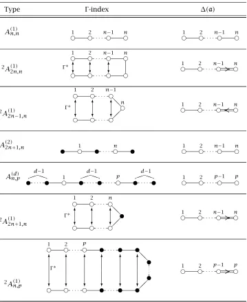
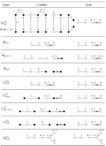
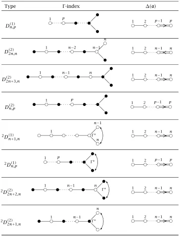
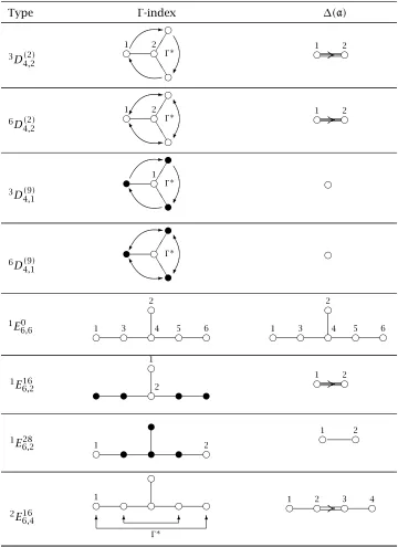
TheΓ-indices forkalgebraically closed, the real numbers, thep-adic numbers, finite fields, and numbers fields have been classified by Tits [Tit66]. In this thesis we will derive algo-rithms to compute the fine structure associated with these Γ-indices. In Table 1 below we list the absolutely irreducibleΓ-indices together with the associated restricted root system. In the table we use the following notation:
LetD =(X,∆,∆0(Γ),[σ ]) be aΓ-index. For theΓ-indices we use the notationgXn,rt . Here
X denotes the type ofΦ(T ), i.e. one ofA, B, . . . , G,nthe rank ofΦ,r the rank of ¯∆Γ andg the order of the action ofΓ on the Dynkin diagram. In the case thatg=1 (i.e. the Dynkin diagram has no nontrivial automorphism) we will omit it in the notation. Finallyt denotes either the degree of the division algebra, which occurs in the definition of the considered form or the dimension of the anisotropic kernel. To differentiate between these two cases we putt between parentheses when it stands for the degree of the division algebra. In fact the degree of the division algebra is only used ifXis of classical type.
Table 2.1:Γ-indices
Type Γ-index ∆(a)
An,n(1) 1e 2e n−e1 ne 1e 2e n−e1 ne
2A(1)
2n,n Γ e6? e6? e6? e
∗ e 1 e 2 e
n−1
e n e 1 e 2 e
n−1
e
n
2A(1)
2n−1,n e e e
e n @ @ 6 ? 6 ? 6 ? Γ∗ e 1 e 2 e
n−1
e
1
e
2
e
n−1
e
n
A(2)2n+1,n u 1e u ne u 1e 2e n−e1 ne
A(d)n,p u u 1e
u u pe u u
d−1 PP
d−1 PP
d−1 PP e 1 e 2 e
p−1
e
p
2A(1)
2n+1,n e e e
u @ @ 6 ? 6 ? 6 ? Γ∗ e 1 e 2 e n e 1 e 2 e
n−1
e
n
2A(1)
n,p e e e u u u
u u @ @ 6 ? 6 ? 6 ? 6 ? 6 ? 6 ? Γ∗ e 1 e 2 e p
u u u
e
1
e
2
e
p−1
e
p
Table 2.1:continued
Type Γ-index ∆(a)
2A(d) n,p
d|(n+1) u u e u u e u u
u u @ @ 6 ? 6 ? 6 ? Γ∗ 6 ? 6 ? 6 ? 6 ? 6 ?
u u 1e u u pe u u
d−1 PP
d−1 PP e 1 e 2 e
p−1
e p Bn,n e 1 e 2 e
n−1
e n e 1 e 2 e
n−1
e
n
Bn,n−1
e
1
e
2
e e n−e1 u 1e 2e n−e2 n−e1
Bn,p 1 2
e e pe u u u 1e 2e p−e1 pe
Cn,n(1) 1e 2e n−e1 ne 1e 2e n−e1 ne
C2n,n(2)
u 1e u n−e1 u ne 1e 2e n−e1 ne
C2n(2)+1,n u 1e u n−e1 u ne u 1e 2e n−e1 ne
Cn,p(2) u 1e
u pe u u u 1e 2e p−e1 pe
D(1)n,n e
1
e
2
e
n−3
e
n−2
e
n−1
@@ne
e
1
e
2
e
n−3
e
n−2
e
n−1
@@ne
Table 2.1:continued
Type Γ-index ∆(a)
D(1)n,p
e 1 e p u u u
@@u
e
1
e
2
e
p−1
e
p
D2n,n(2) u e
1
u n−e2 u n−e1 e n @ @u e 1 e 2 e
n−1
e
n
D(2)2n+3,n
u 1e u n−e1 u ne u u @ @u e 1 e 2 e
n−1
e
n
D(2)n,p
u 1e u pe u u
u @ @u e 1 e 2 e
p−1
e
p
2D(1)
n+1,n e e 1
e e e
e
n−1
@ @e n Γ∗ ] e 1 e 2 e
n−1
e
n
2D(1) n,p e 1 e p u u u
@@u Γ∗ ] e 1 e 2 e
p−1
e
p
2D(2) 2n+2,n
u 1e u n−e1 u ne u
@@u Γ∗ ] e 1 e 2 e
n−1
e
n
2D(2)
2n+1,n u e 1
u n−e1 u e n @ @e Γ∗
] 1e 2e n−e1 ne
Table 2.1:continued
Type Γ-index ∆(a)
3D(2) 4,2 e e e T Te Γ∗ K 2 1 e 1 e 2
6D(2) 4,2 e e e T Te Γ∗ K -M 2 1 e 1 e 2
3D(9) 4,1 u e u T Tu Γ∗ K 1 e
6D(9) 4,1 u e u T Tu Γ∗ K -M e
1E0
6,6 1e
e 3 e4 e 2 e 5 e 6 e 1 e 3 e4 e 2 e 5 e 6
1E16
6,2 u u e2
e
1
u u e
1
e
2
1E28
6,2 1e
u u
u
u 2e
e
1
e
2
2E16 6,4 e 1 e e e e e Γ∗
6 6 6 6
e 1 e 2 e 3 e 4
Table 2.1:continued
Type Γ-index ∆(a)
2E160
6,2
e u u
e
1
u 2e
Γ∗
6 6 6 6
e
1
e
2
2E1600
6,2
u u e2 e
1
u u
Γ∗
6 6 6 6
e
1
e
2
2E29 6,1 e 1 u u u u e Γ∗
6 6 6 6
e
2E35 6,1
u u u
e
1
u u
Γ∗
6 6 6 6
e
E7,70
e 1 e 3 e4 e 2 e 5 e 6 e 7 e 1 e 3 e4 e 2 e 5 e 6 e 7
E7,49
e 1 e 2 e3 u
u 4e u e
1 e 2 e 3 e 4
E7,328
e
1
u u
u
u 2e 3e e
3
e
2
e
1
E7,231
u 1e u u
u u 2e e
1
e
2
Table 2.1:continued
Type Γ-index ∆(a)
E8,80 e 1 e 3 e4 e 2 e 5 e 6 e 7 e 8 e 1 e 3 e4 e 2 e 5 e 6 e 7 e 8
E8,428 e
4
u u
u
u 3e 2e 1e e
1 e 2 e 3 e 4
F4,40
e 1 e 2 e 3 e 4 e 1 e 2 e 3 e 4
F4,121
u u u 1e e
G2,20
e 1 e 2 e 1 e 2
2.11
θ-index
In this section we apply the results to the case of symmetric spaces. In particular, we discuss the index associated with an involutorial automorphism of a reductive algebraic group. Let
Gbe a reductive algebraic group,θ∈Aut(G)an involution andT aθ-stable maximal torus ofG. WriteX=X∗(T ),Φ=Φ(T )and letE
θ = {1,−θ} ⊂Aut(X,Φ)be the subgroup spanned by−θ|T. In this case we will also writeX0(θ), ¯Xθ,Φ0(θ), ¯Φθ,W1(θ), ¯Wθ,∆0(θ), ¯∆θ instead of, respectively,X0(Eθ), ¯XEθ,Φ0(Eθ), ¯ΦEθ,W0(Eθ), W1(Eθ), ¯WEθ,∆0(Eθ), ¯∆Eθ. AEθ-order on X will also be called a θ-order on X, a Eθ-basis of Φ a θ-basis ofΦ and a Eθ-index a
θ-index.
Let ∆ be a θ-basis of Φ. To find the θ-index we need to find the action of [−θ] on
−w0(θ)θ. Thenθ∗=[−θ]. Note thatθ∗(∆)∈Aut(X,Φ,∆)= {φ∈Aut(X,Φ)|φ(∆)=∆},
θ∗(∆)2=id andθ∗(∆
0(θ))=∆0(θ).
The indices of involutions of(X,Φ)can be easily determined using the following result from [Hel88]:
Lemma 4([Hel88, Lemma 2.14]). Let∆be a basis ofΦ,∆0⊂∆a subset andθ∗∈Aut(X,Φ,∆) such thatθ∗(∆
0)=∆0,(θ∗)2=id. LetX0be theZ-span of∆0inXandΦ(∆0)=Φ∩X0. Then there is an involutionθ ∈Aut(X,Φ)with index(X,∆,∆0, θ∗)if and only ifθ∗|∆0=id∗(∆0)
(the opposition involution of∆0with respect toΦ(∆0)).
Remark 6. The above θ-index may depend on the choice of theθ-basis. However ifTθ− is a maximal θ-split torus, then by [Ric82, 4.7] ¯Φθ = Φ(Tθ−) is a root system and by Propo-sition 3 the θ-index does not depend on theθ-basis. Combined with the conjugacy of the maximalθ-split tori underG0θit follows now that theθ-index is uniquely determined by the
G-isomorphism class ofθ:
Proposition 5([Hel88]). LetAbe a maximalθ-split torus ofG,T ⊃Aa maximal torus and∆
aθ-basis ofΦ(T ). Theθ-index(X,∆,∆0,θ∗)is uniquely determined (up to congruence) by the isomorphy class ofθ.
Remark 7. Theθ-indices were classified in [Hel88]. Algorithms for the corresponding fine structures were given in [Fowler03]. Some of the cases discussed there overlap with cases discussed in this thesis. Those would be cases such that|Γ| =2. However, not all cases such that|Γ| =2 occur asθ-indices.
Remark 8. For symmetric k-varieties, there exists a similar index, which is a combination of the aboveΓ-index and θ-index. This is called a Γθ-index and is again determined up to congruence by the isomorphy class of the symmetrick-variety.
2.12
Root Space Decomposition
space decomposition corresponding to a maximalk-split torus, and for aθ-split or a(θ, k) -split torus as well.
LetAbe a maximalk-split torus ofG,athe Lie algebra ofA, andgthe Lie algebra ofg. Then:
g=g0⊕
X
λ∈Φ(A)
gλ.
HereΦ(a)is the root system ofaing. LetT ⊃Abe a maximalk-torus withtits Lie algebra andΦ(t)its root system. LetΦ(λ)= {α∈Φ(t)|α|a=λ}. Then we have the following result:
Theorem 2.2. Letg,a,t,Φ(t), andΦ(a)be as above. Then:
(1) g0=Zg(a)=t⊕
X
α∈Φ0(Γ)
gα.
(2) g=Zg(a)⊕
X
λ∈Φ(a)
gλ,withgλ=Pα∈Φ(λ)gα.
Chapter 3
The Algorithm
The computation depends on the original choice of basis for the Lie algebragand the choice of theΓ-basis forΦ:=Φ(t). Γ is the Galois group of a finite splitting extensionK ofkfor a maximalk-torusT,∆= {α1, . . . , αn}is aΓ-basis ofΦ,∆0is the set ofα∈∆that project to 0, and ¯∆:=π (∆−∆0)= {λ1, . . . , λr}is the restricted basis.
3.1
Step One:
Using theΓ-index, determine the elements ofΓ.
3.2
Step Two:
Find a basis of the restricted root system in terms of the basis of the original root system by finding the projection of eachαj ∈∆,and determine eachλiin terms ofαj.
3.3
Step Three:
Note the type of restricted root system, and determine a representativewi ∈WΓ for each
sλi, withλi ∈∆¯. This gives representatives of the Weyl group of Φ(a)in the Weyl group of
3.4
Step Four:
DetermineΦ(λi):= {α∈Φ|π (α)=λi}for eachλiin Step One.
3.5
Step Five:
Find the roots inΦ(a)+using the Weyl group as determined in step 3.
3.6
Step Six:
We are interested in the structure of Φ(a). Note that Φ(−λ) = −Φ(λ), so it suffices to determineΦ(λ)for λ∈Φ(a)+. Do this using the fact thatλ =w(λi)for somew ∈W (a),
Chapter 4
Techniques used for Computing the Bases and Weyl
Groups
The first steps in the algorithm involve determining the Weyl group elementwσ as in 1.6 in order to recover the action ofΓ. We also refer towσ aswσ(Γ). In most cases, this element is determined by considering that forαnot in∆0,wσj(α)=αfor somej, and that forαin
∆,wσj(α)=0 for that samej. Recall thatσ =wσ[σ ]. We then find the projection of each
αusingπ (α)= |Γ1|Σσ∈Γσ (α), which will be ourλi. By obtainingλi in terms ofαj, we find a basis of the restricted root system in terms of the basis of the original root system. For
αj ∈∆0, the projection is always 0.
In the following I list the type of Γ-index, the elements of the Galois group Γ, and give the nontrivial projectionsπ (αi), which give us the basis ¯∆ofΦ(a). In doing this, the first two steps of the algorithm are completed.
4.1
A cases
4.1.1 TypeA(1)n,n e 1 e 2 e
n−1
e
n
Γ = {id}
λi=π (αi)=αi
Here, nothing is fixed byΓ. Therefore, every root projects down to itself and∆(t)=∆(a).
4.1.2 Type2A(1) 2n,n
e e e e
6 ? 6 ? 6 ? Γ∗ e 1 e 2 e
n−1
e
n
Γ = {id, σ} σ =σ∗
λi=π (αi)=π (α2n−i+1)= 12(αi+α2n−i+1)
4.1.3 Type2A(1) 2n−1,n
e e e
e n @ @ 6 ? 6 ? 6 ? Γ∗ e 1 e 2 e
n−1
Γ = {id, σ} σ =σ∗
λi=π (αi)=π (α2n−i)=12(αi+α2n−i)
Forλiin∆(a)withi=1,· · ·, n−1, notice that there are two base roots that project down toλi.
4.1.4 TypeA(2)2n+1,n
u 1e u ne u
σ =s1s3...s2n+1
λi=π (αi)=12(α2i−1+2α2i+α2i+1)
α2i−1is fixed fori=1,· · ·, n+1 . The rootsα2i−1project down to zero and the rootsα2i project down toλi=12(α2i−1+2α2i+α2i+1).
4.1.5 TypeA(d)n,p
u u 1e u u pe u u
d−1 PP
d−1 PP
d−1 PP
Γ = {id, σ ..., σd−1}
σ =sαd−2sαd−3...sα2sα1sα2sα3...sαd−2sαd−1sα2d−2sα2d−3...sαd+2sαd+1sαd+2sαd+3...sα2d−2sα2d−1
...sαpd−2sαpd−3...sα(p−1)d+2sα(p−1)d+1sα(p−1)d+2sα(p−1)d+3...sαpd−2sαpd−1sαpd+1sαpd+2sαpd+1
sαpd+3sαpd+2sαpd+1...sαnsαn−1...sαpd+2sαpd+1
λi=π (αdi)= 12(αd(i−1)+1+αd(i−1)+2+...+2αdi+αdi+1...+αd(i+1)−2+αd(i+1)−1)
Example4.1. Let us consider theΓ-diagram:
u u e u u e u u
In this case,Γ = {id, σ}, andσ2=id.
σ =s1s2s1s4s5s4s6s7s6.
λ1=π (α3)= 12(α1+α2+2α3+α4+α5)
λ2=π (α6)= 12(α4+α5+2α6+α7+α8).
4.1.6 Type2A(1) 2n+1,n
e e e
u
@@ 6
? 6
? 6
? Γ∗
e
1
e
2
e
n
λi=π (αi)=π(α2n−i+2)=12(αi+α2n−i+2)
λn=π (αn)=π (α2n−i+2)= 12(αn+αn+1+αn+2)
4.1.7 Type2A(1) n,p
e e e u u u
u u @@ 6 ? 6 ? 6 ? 6 ? 6 ? 6 ? Γ∗ e 1 e 2 e p
u u u
Γ = {id, σ}
σ =sαp+1sαp+2sαp+1sαp+3sαp+2sαp+1· · ·sαp+msαp+m−1· · ·sαp+1σ ∗
(λp)=π (αp)=12(αp+αp+1+...+αp+m+1)
(λi)=π (αi)=π (α(n−i+1)= 12(αi+αn−i+1)
The rootαp+i is fixed fori =1,· · ·, m. Forλiin∆(a)withi =1,· · ·, p−1, notice that there are two base roots that project down toλi.
Remark9. n=p+m
4.1.8 Type2A(d)n,p
u u e u u e u u u
u u @ @ u 6 ? 6 ? 6 ? Γ∗ 6 ? 6 ? 6 ? 6 ? 6 ? 6 ?
u u 1e u u pe u u
d−1 PP
d−1 PP
Γ = {id, σ , σ2, ...σd−1, γ, γ2, ...γd−1, γσ , γσ2, ..., γσd−1, ...γd−1σ , γd−1σ2, ..., γd−1σd−1}
σ =sαd−2sαd−3...sα2sα1sα2sα3...sαd−2sαd−1sα2d−2sα2d−3...sαd+2sαd+1sαd+2sαd+3...
sα2d−2sα2d−1...sαpd−2sαpd−3...sα(p−1)d+2sα(p−1)d+1sα(p−1)d+2sα(p−1)d+3...
sαpd−2sαpd−1sαpd+1sαpd+2sαpd+1sαpd+3sαpd+2sαpd+1...sαpd+msαpd+m−1...sαpd+2sαpd+1σ ∗
γ=sαn−d+3sαn−d+4...sαn−1sαnsαn−1sαn−2...sαn−d+3sαn−d+2sαn−2d+3sαn−2d+4...
sαn−pd−1sαn−pd+dsαn−pd+d−1sαn−pd+d−2...sαn−pd+3sαn−pd+2σ ∗
λi =π (αdi)=π (αn−di+1)= 2d1 (αdi−(d−1)+2αdi−(d−2)+3αdi−(d−3)+...+(d−1)αdi−1+
dαdi+(d−1)αdi+1+(d+2)αdi+2+...+2αdi+(d−2)+αdi+(d−1)+αn−di−d+2+2αn−di−d+3+ 3αn−di−d+4+...+(d−1)αn−di+dαn−di+1+(d−1)αn−di+2+(d+2)αn−di+3+...+2αn−di+(d−1)+
αn−di+d)
λp =π (αpd)=π (αpd+m+1)= 2d1