Comparison of Digital Image Inpainting Techniques Based on SSIM

Comparison of Digital Image Inpainting

Techniques Based on SSIM

Mrs Anupama Sanjay Awati1, Mrs. Meenakshi R. Patil2 Dept of Electronics and communication

KLS Gogte Institute of Technology, Belgaum, JAGMIT, Jamkhandi

Abstract— Digital Image Inpainting is a technique used to repair a damaged region of an image in such a way that it appears natural and continuous to an observer who is seeing it for the first time. Image inpainting is an important research area in the field of image processing used for image editing and image stitching. In this paper we compare two Digital Image Inpainting Techniques by using (structural similarity) SSIM as a metric for comparison. In the first method (Bilateral Image Inpainting. algorithm) the region to be inpainted is convolved with a bilateral kernel obtained by multiplying range and space kernels. The damaged pixel value is replaced by a weighted average of its neighbors in both space and range. A bilateral filter is an edge-preserving smoothing filter. In the second method (gradient based convolution algorithm) the damaged region is reconstructed by convolving the image with an adaptive kernel calculated by gradient of known pixels in the neighborhood of a missed pixel. These techniques are evaluated by writing a MATLAB code and using parameters like PSNR, time required for filling, SSIM, number of damaged pixels and number of reconstructed pixels.

Index Terms: Inpainting, Bilateral filtering, Inpainting using Adaptive Kernel, Structural Similarity.

I. INTRODUCTION

Digital Image Inpainting is an art and science behind reconstructing parts of an image in a visually undetectable way. Inpainting is used in a primitive form in certain image editing software. In Image Inpainting Technique the user specifies the area to be inpainted. This region is filled by using the information available in the surrounding area of the same image. Marcelo Bertalmio, Guillermo Sapiro, were the first authors to propose Digital image inpainting. In paper [7] the authors have proposed inpainting using a Partial difference equation. In paper [1] Manuel M. Oliveira, Brian Bowen, Richard McKenna and Yu-Sung Chang have proposed algorithm based on convolution. In [2] Mohiy M. Hadhoud, Kamel. A. Moustafa and Sameh. Z. Shenoda has proposed a modified convolution based algorithm. In [3] H.Noori , Saeid Saryazdi have prposed a algorithm based on directional median filtering. Paper[6] proposes a median diffusion method by Rajkumar Biradar, And Vinayadattv Kohir. Christine Guillemot and Olivier Olivier Le Meu [9] have proposed a rigorous literature survey with all the algorithm’s , results and comparisons. The algorithms found in literature can be classified as diffusion and non-diffusion, structural and textural, isotropic and anisotropic, geometry based and exemplar based, spatial domain and frequency domain[8] .

In diffusion-based inpainting, the information surrounding the damaged region is propagated into the damaged regions via lines of equal intensities called as isophotes. The techniques are based on partial differential equations. These methods are advantageous for propagating straight lines, curves, and for inpainting small regions. The disadvantage is that the inpainted region is blurred while recovering large areas.

The exemplar (non diffusion) based techniques help to preserve, propagate and extend linear image structure. Exemplar-based techniques find patches in the rest of the image which are similar to the patch to be filled, and then the most similar patch is copied in the missing region. This mechanism preserves image isophotes of the known parts of a target patch. Filling order is critical, and has a large impact on the resulting quality. The algorithm first estimates the importance, or priority of our current boundary pixels of the region to be inpainted, with respect to image isophotes. It then finds the border pixel with the largest priority and copies the missing information by finding a similar patch from the source regions. The disadvantage is that the reconstructed image is annoying when the source region does not contain similar patch. The algorithm is not designed to handle curved structures.

In order to understand the algorithms we need to understand the terms used in image inpainting literature. The original image is described as I, the area that has to be inpainted is denoted as Ω ,the border of this region and the known region also known as source region is indicated by ф. This is shown in Figure

©IJRASET 2014: All Rights are Reserved

498

II. INPAINTING TECHNIQUES A. Gradient based Convolution Algorithm

A gradient based convolution algorithm is proposed by Noori et al. [5]. The main idea of the proposed convolution based inpainting algorithm, is to use an adaptive kernel permitting a better processing edge regions. The gradient of known pixels in the neighborhood of a missed pixel is used to compute weights in convolving mask. Since gradient values in edge regions are large, and contribution of pixels adjacent of edges should be less than contribution of pixels in smooth regions, the weights are computed by a predefined function of the image gradient. Small weights are assigned to missed pixels' in the neighborhood of pixels with large local gradients, edges are preserved better. The weights of convolution mask changes adaptively with gradient of pixels in a neighborhood. Thus, the algorithm can estimate missed pixels while preserve sharp edges in image.

The gradient of the pixels in a small neighborhood is obtained and a function is defined by the equation

F(xk) = 1 − ( ) if x≤ α/2 (1)

F(xk) = ( − 1) if ≤ x ≤ α F(xk) = 0 i f x≥α The weights of convolution mask are defined as ( ) = F(xk) (2)

The damaged pixel is estimated by using the following equation ( ) = (1 − ∑ (( )) ( ) + ∑ (( ) ( ) (3)

where f'(p) is estimated value, f(k) is value of a known pixel in the current neighborhood, n is the number of known pixel in the current neighborhood. Where x is gradient value of the current pixel in the image, α is a parameter giving an estimation of the missed pixel gradient and it control the softness of propagation. B. Bilateral Image Inpainting. Algorithm A convolution based technique using bilateral filtering is proposed by [4],[7]. A bilateral filter is an edge-preserving smoothing filter. The bilateral filter replaces a pixel's value by a weighted average of its neighbors in both space and range. This is applied as two Gaussian filters at a localized pixel neighborhood, one in the spatial domain, and the other in the intensity domain. This approach permits preserves sharp edges. Every sample pixel value is replaced by a weighted average of its neighbors. The bilateral filters are efficient in denoising, and hence can be used to inpaint by estimating the lost (damaged) pixel value by its neighbors. Inpainting is proposed using a convolution with a bilateral averaging kernel. Image Inpainting is carried out by using a bilateral filter which preserves the edges and also provides smoothing. The bilateral filter takes a weighted sum of the pixels in a local neighborhood; the weights depend on both the spatial distance and the intensity distance. Thus edges are preserved well while noise is averaged out. For smooth regions, pixel values in a small neighborhood are similar to each other, and the bilateral filter acts as a domain filter. When the bilateral filter is centered on a pixel on the bright side of the boundary, the kernel function assumes values close to one for pixels on the same side, and values close to zero for pixels on the dark side. For every pixel, the kernels are calculated using its neighbors in both space and range domains to implement bilateral filtering. The range coefficients are modified by using the gradient of the image to be inpainted rather than difference in pixel value. Let Ω be the damaged area to be inpainted and ∂Ω be its one-pixel thick boundary. The algorithm consists of convolving the region to be inpainted with a bilateral kernel obtained by multiplying range and space kernels. Every sample is replaced by a weighted average of its neighbors. Let I and If represent the input and filtered signal respectively, p is current pixel (position), q is neighbor pixel, w(p, q) is a weight devoted to pixel q ,ds is the Euclidian distance, σd and σr are two user defined numbers that denote geometric and photometric spread and (xp, yp) and (xq, yq) are coordinates of pixels p and q, respectively. Let p be the damaged pixel to be inpainted and q presents its undamaged neighbor pixel and Pdir is the spatial vector from q to p. The damaged pixel can be approximated by equation 3 = ( , ) ( ) ( , ) (4)

( , ) = 1( . ) 2( , ) (5)

1( . ) = / (6)

2( , ) = / .∇ (7)

Pdir = [ − − ] (9) There are two parameters that control the behavior of the bilateral filter are σd(geometric spread) and σr(photometric spread) which characterize the spatial and intensity domain behaviors, respectively. Both σd and σr determine the level of smoothness. Assigning σr to zero reduces the bilateral filter to a simple Gaussian smoothing filter with a cut-off frequency proportional to 1/ σd. Hence smaller values of σd better preserve fine details and edges. The size of the window must be determined in such a manner that at least one known pixel exists in the window region at the first iteration. A small value of σd causes a small considered neighborhood and therefore the inpainting process needs more iterations and only a small part of the damaged area will be reconstructed. A large value of σd will provide a blurring effect in both texture and structure regions. A midrate value of σd can inpaint the missed region adequately.

III. IMPLEMENTATION

In this paper we have implemented and compared techniques proposed by Noori et al, namely Bilateral Image Inpainting algorithm and Gradient based Convolution Algorithm, for various damaged input images. The algorithms are as stated below

A. Bilateral Image Inpainting. algorithm

Bilateral Filter can be used to estimate the lost (damaged) pixel value from its neighbors. The can be done by obtaining a bilateral averaging kernel for a neighborhood of size w. The space domain kernel is found by equation 3 and range domain kernel is found by equation 4.The algorithm is implemented by convolving the region to be inpainted with a bilateral kernel obtained by multiplying range and space kernels. A damaged pixel is replaced by a weighted average of its neighbors

Step1: Identify the regions to be inpainted. Step2: Estimate w1 by equation 6. Step3: Estimate w2 by equation 7.

Step4: Calculate w as product of w1 and w2.

Step6: Estimate the value of damaged pixel using equation 1. Step7: Repeat the above steps for fixed number of

iterations.

B. Gradient based Convolution Algorithm

Step1. The region of the colored image to be inpainted is identified.

Step2. The colored image is decomposed into the corresponding RGB components. Step3. The gradient of the pixels in a small neighborhood is obtained

Step4. A function is defined by the equation 1.

Step5. The weights of convolution mask are calculated by using the equation 2. Step6. The damaged pixel is estimated by using equation 3in each plane.

Step7. The colored image is reconstructed by combining the pixels of the corresponding RGB components

The performance of the algorithm are evaluated by Structural Similarity(SSIM) proposed by Hamid Amiri et al[10]. If x and y are the original and reconstructed images and µx, µy denote the average of x and y respectively . σx ,σy refer to the

variance of x and y respectively and σxy is the cross covariance between x and y the constants c1, c2, are employed to stabilize

the metric for the case where the means and variances become small. The parameters c1=0.01*2552 c2=0.03*2552. The SSIM index is then given by :

( , ) = 2 + (2 + )

+ + ( + + )

IV. RESULTS

The discussed algorithms are tested on a variety of images to investigate the performance of inpainting. The test set constitutes of Standard images used by image processing community. The original images are clean images, and these images are artificially degraded by drawing random lines on them. The random lines are treated as scratches or areas of inpainting. These degraded images are then inpainted. The comparison of algorithms is carried out by implementing in MATLAB R2014. In our study, the quantitative valuation is performed by calculating peak signal to noise ratio (PSNR) and is defined as

= 20 255/ ( , )

©IJRASET 2014: All Rights are Reserved

500

where u is original image, v is inpainted image and M × N is size of u and v. Table 1 to3 show Time elapsed, PSNR, SSIM, number of damaged pixels and number of reconstructed pixels for number of iterations equal to 100. (Bilateral Image Inpainting for five images). The images are downloaded from net. Figure 2 to Figure 11 show the damaged and reconstructed images for Bilateral Image Inpainting. Table 4 and 5 show Time elapsed, PSNR, SSIM, number of damaged pixels and number of reconstructed pixels for number of iterations equal to 100.( Gradient based Convolution Algorithm for three images) Figure12 to Figure 17 show the damaged and reconstructed images for Gradient based Convolution Algorithm. Table 6 show the compaision results for Bilateral Image Inpainting Algorithm and Gradient based Convolution Algorithm. From the images we see that the reconstructed images are blurred

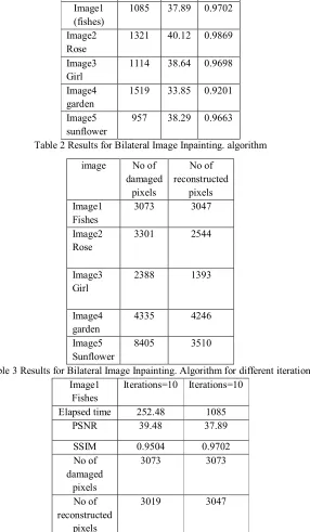
Table 1Results for Bilateral Image Inpainting. algorithm

Image Elapsed

time

PSNR SSIM

Image1 (fishes)

1085 37.89 0.9702

Image2 Rose

1321 40.12 0.9869

Image3 Girl

1114 38.64 0.9698

Image4 garden

1519 33.85 0.9201

Image5 sunflower

957 38.29 0.9663

Table 2 Results for Bilateral Image Inpainting. algorithm

image No of

damaged pixels No of reconstructed pixels Image1 Fishes

3073 3047

Image2 Rose

3301 2544

Image3 Girl

2388 1393

Image4 garden

4335 4246

Image5 Sunflower

8405 3510

Table 3 Results for Bilateral Image Inpainting. Algorithm for different iterations Image1

Fishes

Iterations=10 Iterations=10

Elapsed time 252.48 1085

PSNR 39.48 37.89

SSIM 0.9504 0.9702

No of damaged

pixels

3073 3073

No of reconstructed

pixels

Fig2 Damaged Rose. Fig 3 Reconstructed Rose.

Fig 4. Damaged Fishes Fig 5. Recontructed Fishes

Fig 6. Damaged Girl Fig 7. Reconstructed Girl

Fig 8. Damaged Garden Fig 9. Reconstructed Garden

502

Fig12 Damaged Flowers Fig13 Reconstructed Flower

Fig14 Damaged Forest Fig15 Reconstructed Forest

Fig16 Damaged Garden Fig17 Reconstructed Garden

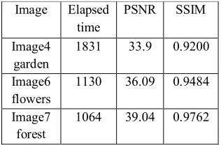
Table 4 Results for Gradient based Convolution Algorithm

Image Elapsed

time

PSNR SSIM

Image4 garden

1831 33.9 0.9200

Image6 flowers

1130 36.09 0.9484

Image7 forest

1064 39.04 0.9762

Table 5 Results for Gradient based Convolution Algorithm

image No of

damaged pixels

No of reconstructed

pixels Image4

garden

4335 4246

Image6 flowers

11258 8822

Image7 forest

Table 6 Results for Bilateral Image Inpainting Algorithm and Gradient based Convolution Algorithm Image1 Fishes Bilateral Image Inpainting. Algorithm Gradient based Convolution Algorithm

Elapsed time 1519 1831

PSNR 33.85 33.9

SSIM 0.92 0.92

No of damaged

pixels

4335 4335

No of reconstructed

pixels

4246 4246

From Table 1 we see that SSIM is highest for Rose image. From Table 4 we see that SSIM is highest for forest image. Table 6 indicates for same SSIM Gradient based convolution takes more time. Table 2 and 5 show the number of pixels which can be reconstructed by increasing the number of iterations. Table 3 indicates the performance for Bilateral Image Inpainting for different values of iterations,

V. CONCLUSION

The results of bilateral filtering and Noori et al’s Algorithm, are presented in this paper. The performance can be compared on the basis of PSNR, SSIM, number of reconstructed pixels and time required. Bilateral filtering takes less time for reconstruction and generates a good PSNR. Sometimes PSNR metric is misleading, but SSIM indicates the performance in a better way. In future the algorithms can be tested for different iterations and values of σd and σr. The algorithm’s can be implemented for Object Removal application of Digital Image Inpainting.

REFERENCES

[1] Manuel M. Oliveira, Brian Bowen, Richard McKenna and Yu-Sung Chang, “ Fast Digital Image Inpainting” Imaging and Image Processing (VIIP 2001), Marbella, Spain, September 3-5, 2001.

[2] Mohiy M. Hadhoud, Kamel. A. Moustafa and Sameh. Z. Shenoda, “Digital Images Inpainting using Modified Convolution Based Method “,International journal of signal processing , image processing and pattern recognition .

[3]H.Noori , Saeid Saryazdi,” Image Inpainting using Directional Median Filters”, Shahid Bahonar University of Kerman.2010 International conference on computational Intelligence and communication network.

[4]. H. Noori, , S. Saryazdi and H. Nezamabadi-Pour,“ABilateral Image Inpainting”, IJST, Transactions of Electrical Engineering, Vol. 35, No. E2, pp 95-108, 2011, printed in the Islamic Republic of Iran, Shiraz University.

[5]Noori H,Saryazdi S and Nezamabadi-pour H 2010 “A convolution based image inpainting”, In the 1st

International Conference o n Communication and Engineering, University of Sistan & Baluchestan,December.

[6]RAJKUMARL BIRADAR, and VINAYADATTV KOHIR “A novel image inpainting technique based on median Diffusion”. [7] Marcelo Bertalmio, Guillermo Sapiro, Vicent Caselles and Coloma Ballester, “Image Inpainting”, SIG- GRAPH 2000.

[8]. ABilateral Image Inpainting, H. Noori, S. Saryazdi and H. Nezamabadi-Pour, IJST, Transactions of Electrical Engineering, Vol. 35, No. E2, pp 95-108, 2011.

[9]Christine Guillemot and Olivier Olivier Le Meu Image “Inpainting Overview and recent advances”, 1053-5888/14/$31.00©2014IEEE IEEE SIGNAL PROCESSING MAGAZINE [127] JANUARY 2014.