ABSTRACT
HARTFORD, ALAN HUGHES. Computational approaches for maximum likelihood estimation for nonlinear mixed models. (Under the direction of Marie Davidian and John F. Monahan).
converge to a solution.
A method must provide good estimates of the likelihood at points in the param-eter space near the solution. This work compares this ability among the numerical integration techniques, Gaussian quadrature, importance sampling, and Laplace's ap-proximation. A new \scaled" and \centered" version of Gaussian quadrature is found to be the most accurate technique. In addition, the technique requires evaluation of the integrand at only a few abscissas. Laplace's method also performs well; it is more accurate than importance sampling with even 100 importance samples over two dimensions. Even so, Laplace's method still does not perform as well as Gaussian quadrature. Overall, Laplace's approximation performs better than expected, and is shown to be a reliable method while still computationally less demanding.
ii
To my brother and sisters,
iii
Biography
iv
Acknowledgements
Thanks to all of the following people. Without you this would not have been possible.
To my advisors, Dr. John Monahan and Dr. Marie Davidian, for your
instruc-tion and patience.
To my committee members, Professors Sastry Pantula, Pierre Gremaud, and
Carla Savage, for actually reading all of this.
To Jenny Langdon who has been a constant, unwaivering support.
To the friends I have made at NCSU and UNL: Erin Blankenship, Ann Oberg,
Sarah Hardy, Jennifer Ho, Dawn Haines, Jennifer Mueller, Valerie Shostrom, Carlos Silva, Anne Parkhurst and most especially, Gordon Brown.
To Terry Byron and Nalin Dahyabhai for going beyond the call of duty. They
made my computing life so much easier.
To Dr. Carol Gotway, Dr. J.-C. Lu, and Stew Williams for the wonderful
research opportunities they shared with me.
Special thanks to my parents, grandparents, brother, sisters, and the rest of my
v
Contents
List of Figures
vii
List of Tables
ix
1 Introduction
1
1.1 Motivation . . . 1
1.2 Model . . . 3
1.3 Approximate Methods . . . 4
1.3.1 First Order Linearization . . . 5
1.3.2 Laplace's Approximation . . . 7
1.3.3 Importance Sampling . . . 11
1.3.4 Gaussian Quadrature . . . 13
1.4 Preview of Results . . . 15
2 Consequences of Misspecifying Assumptions in Nonlinear Mixed
Ef-fects Models
17
2.1 Introduction . . . 192.2 Nonlinear mixed eects model . . . 23
2.3 Approximate methods . . . 27
2.4 Design of simulations . . . 34
2.5 Results . . . 40
2.6 Discussion . . . 48
3 Comparison of Numerical Integration Methods
67
3.1 Introduction . . . 673.2 Integration Methods . . . 70
3.2.1 Laplace's Approximation . . . 70
3.2.2 Importance Sampling . . . 74
3.2.3 Gaussian Quadrature . . . 79
vi
3.4 Sampling the Parameter Space . . . 85
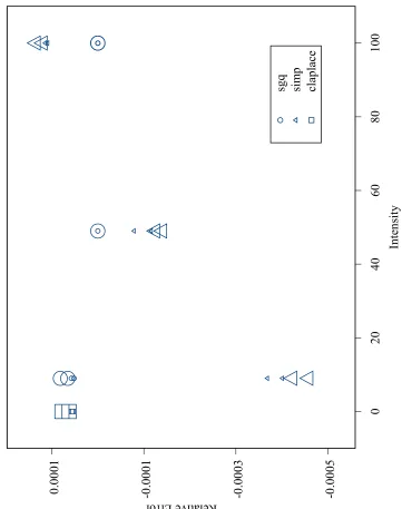
3.5 Results . . . 87
3.5.1 Analysis for Model 1 . . . 90
3.5.2 Analysis for Model 2 . . . 94
3.5.3 Analysis for Model 3 . . . 99
3.5.4 Summary . . . 101
4 Computational Framework for Maximum Likelihood Estimation 120
4.1 Introduction . . . 1204.2 The Model . . . 124
4.3 Integration Method . . . 125
4.4 Initial Estimation . . . 129
4.5 Optimization via a Heuristic Variation on Stochastic Approximation . 132 4.6 Simulation for a Linear Model . . . 134
4.6.1 Model . . . 134
4.6.2 Results . . . 135
4.7 Simulation for a NLMM . . . 137
4.7.1 Model . . . 137
4.7.2 Results . . . 139
4.8 Discussion . . . 139
5 Conclusions and Future Work
141
6 Bibliography
145
A Appendices
147
A.1 \"{Method for Finding Approximate Variances . . . 147A.2 Standard Errors for Approximations using Importance Sampling . . . 150
vii
List of Figures
2.1 Perspective plots of the joint density functions corresponding to the
asymmetric (A) and bimodal (B) random eects distributions. . . 55
2.2 Boxplots of estimates of 1 from data sets for which both methods converged in each panel for each random eects distribution, correct inter-individual model tted. Estimates have been centered and scaled by the true value so that 0 represents no bias and the vertical axis represents bias relative to the truth. Multiplying the numbers on the vertical axis will result in relative percentages. The white bar repre-sents the median, the horizontal bars represent the extremes. In some cases, outliers that distorted the comparison have been deleted; the relative dierence of these estimates from the truth is given numerically. 56 2.3 Same as Fig. 2.2 for 3. . . 57
2.4 Boxplots of estimates of D11 from data sets for which both methods converged in each panel for each random eects distribution, correct inter-individual model tted. Estimates have been centered and scaled as in Fig. 2. The white bar represents the median, the horizontal bars represent actual estimates. In some cases, outliers that distorted the comparison have been deleted; the relative dierence of these estimates from the truth is given numerically. . . 58
2.5 Same as Fig. 2.4 for D12. . . 59
2.6 Same as Fig. 2.4 for D22. . . 60
2.7 Same as Fig. 2.4 for . . . 61
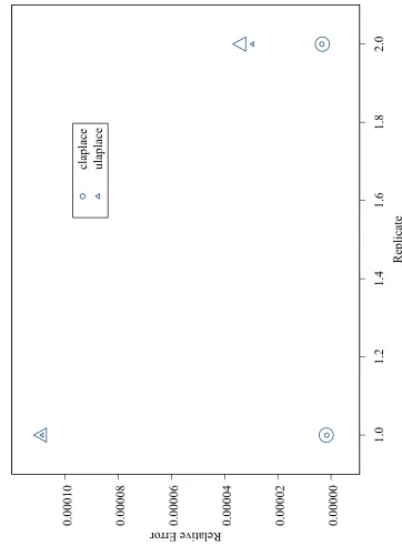
3.1 Model 1, Means of Relative Error for the Laplacian Methods . . . 102
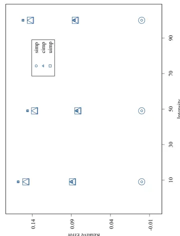
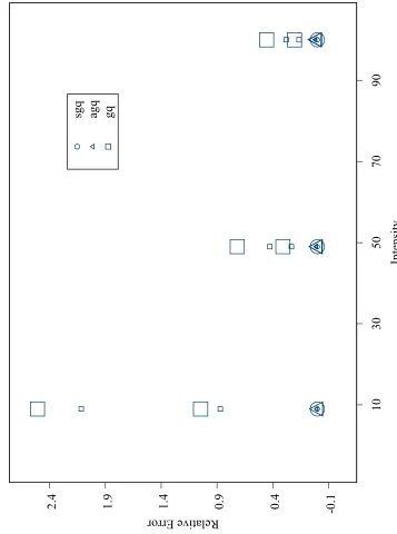
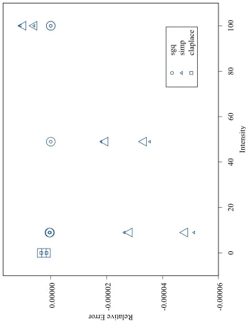
3.2 Model 1, Means of Relative Error for the Importance Sampling Methods103 3.3 Model 1, Means of Relative Error for the Gaussian Quadrature Methods104 3.4 Model 1, Means of Relative Error for the Gaussian Quadrature Meth-ods without gq . . . 105
viii
3.7 Model 2, = 0:15, Means of Relative Error for the Importance Sam-pling Methods . . . 108 3.8 Model 2, = 0:15, Means of Relative Error for the Gaussian
Quadra-ture Methods . . . 109 3.9 Model 2, = 0:15, Means of Relative Error for the Best Methods . . 110 3.10 Model 2, = 0:30, Means of Relative Error for the Laplacian Methods 111 3.11 Model 2, = 0:30, Means of Relative Error for the Importance
Sam-pling Methods . . . 112 3.12 Model 2, = 0:30, Means of Relative Error for the Gaussian
Quadra-ture Methods . . . 113 3.13 Model 2, = 0:30, Means of Relative Error for the Best Methods . . 114 3.14 Model 3, Means of Relative Error for the Laplacian Methods . . . 115 3.15 Model 3, Means of Relative Error for the Importance Sampling Methods116 3.16 Model 3, Means of Relative Error for the Gaussian Quadrature Methods117 3.17 Model 3, Means of Relative Error for the Best Gaussian Quadrature
ix
List of Tables
2.1 Rate of nonconvergence out of 1000 trials for each distribution,
sam-pling scheme, and tting method, correct inter-individual model. . . . 62
2.2 Rate of nonconvergence out of 1000 trials for each distribution, sam-pling scheme, incorrect inter-individual model. . . 63
2.3 Relative Eciency of the First Order method relative to the Laplace method, correct inter-individual model with 2 = 0. Each entry is based on all data sets for which convergence was achieved for both methods. Entries are given in italics in cases where both methods performed poorly (see Figs. 2{7). . . 64
2.4 Performance of Wald and Likelihood Ratio Tests on trials that con-verged for both the full and reduced models, correct inter-individual model. . . 65
2.5 Performance of Wald and Likelihood Ratio Tests on trials that con-verged for both the full and reduced models, incorrect inter-individual model. . . 66
3.1 Abbreviations for the Methods . . . 90
3.2 Model 1, mean relative error. . . 91
3.3 Analysis of Variance for Model 1 . . . 93
3.4 Model 2 ( = 0:15), mean relative error. . . 94
3.5 Analysis of Variance for Model 2 with = 0:15 . . . 96
3.6 Model 2 ( = 0:3), mean relative error. . . 97
3.7 Analysis of Variance for Model 2 with = 0:30 . . . 98
3.8 Model 3, mean relative error. . . 99
3.9 Analysis of Variance for Model 3 . . . 100
4.1 Results for a Linear Model, R2 and Eigenvalues . . . 136
4.2 Results for a Linear Model, Estimates . . . 136
x
A.1 Simulation results for intensive Normal data for testing size. . . 152
A.2 Simulation results for intensive Normal data for testing power. . . 153
A.3 Simulation results for intensive t data for testing size. . . 154
A.4 Simulation results for intensive t data for testing power. . . 155
A.5 Simulation results for intensive Contaminated Normal data (with = :05) for testing size. . . 156
A.6 Simulation results for intensive Contaminated Normal data (with = :05) for testing power. . . 157
A.7 Simulation results for intensive Contaminated Normal data (with = :10) for testing size. . . 158
A.8 Simulation results for intensive Contaminated Normal data (with = :10) for testing power. . . 159
A.9 Simulation results for intensive Asymmetric data for testing size. . . . 160
A.10 Simulation results for intensive Asymmetric data for testing power. . 161
A.11 Simulation results for intensive Bimodal data for testing size. . . 162
1
Chapter 1
Introduction
1.1 Motivation
2
numerically integrate out the random eects and maximize the resulting likelihood function.
The work presented here investigates the performance of methods that approxi-mate the log{likelihood of the NLMM. In Chapter 2, two popular methods for nding estimates for the NLMM are examined. Each method requires normal distributional assumptions on the random eects and intra{individual error. A computer simulation experiment was performed to discover how robust the methods are to these and other assumptions. (Chapter 2 was written as a separate work and is incorporated here in its original form as accepted for publication in Computational Statistics and Data Analysis. Additional tables were added in Appendix A.3 that were not previously included. These tables are not referenced in Chapter 2.)
A second computer simulation, reviewed in Chapter 3, compares several meth-ods used in common practice to approximate the log{likelihood in terms of accuracy and computing time. With the advance of today's computing, another, more com-putationally intense method can be considered. This method is based on maximum likelihood and does not attempt to nd a closed form solution of the likelihood. The likelihood can be numerically integrated and maximized using stochastic approxima-tion, resulting in estimation of parameters based on the true likelihood and not on approximations. This method is described in Chapter 4.
3
methods. These approximate methods, which result in closed form approximate so-lutions to the likelihood, are described in Section 1.3. A preview of the results of Chapters 2{4 is given in Section 1.4 and a nal summary of conclusions and a de-scription of future work is made in Chapter 5.
1.2 Model
Consider the following Hierarchical NLMM,
yij =f(xij;i) +eij (1.1)
(eiji)[0;Ri(i;)]
i =d(ai;;bi)
bi (0;D)
whereyij is thejth response for theith individual,i= 1;:::;M; j = 1;:::;ni;xij is the covariate for theith individual for thejth response;i is ap1 random eects vector
for the ith individual; f(xij;i) is a nonlinear scalar mean function which will also be denoted as fj(i), and as a vector mean function f(i) = [f1(i);:::;fni(i)]
T;
the error for the jth response of the ith individual is eij; and Ri is an nini matrix
function of random eectsiand xed eects(q1). Dependence ofion covariates
4
eects (r 1) and latent random eects bi (k 1). The covariance of bi is the
(kk) matrix D.
Let the conditional density ofyi givenbi bep(yijbi) and the density ofbibe(bi):
Combining the unknown xed parameters into one vector, let =h
T;T;vech (D)TiT
:
Then the maximum likelihood estimates for can be found by maximizing in
L() = YM
i=1
Z
p(yijbi)(bi)dbi (1.2)
where M is the number of individuals.
1.3 Approximate Methods
Because the likelihood (1.2) cannot be maximized with a closed form solution for mean functions that are nonlinear in bi, current inferential methods have approxi-mated the likelihood by either approximating the integrand before integrating or ap-proximating the integral with a nite sum (i.e. a numerical integration). Both strate-gies result in closed form expressions for L() with computable values. The methods discussed in this section include First Order Linearization, Laplace's Method, Impor-tance Sampling, and Gaussian Quadrature. These methods all require the assumption that the intra{individual errors and random eects are normally distributed, i.e.
5
1.3.1 First Order Linearization
Sheiner and Beal (1980) approximated the integral (1.2) by approximating the integrand with a Taylor series expansion for f[d(ai;;bi)] about bi = 0 before in-tegration. Note that here i is denoted by d(ai;;bi) to show explicitly how the expansion will be taken in bi. From (1.1), let ei = Ri1=2[d(ai;;bi);]i where
R1=2
i [d(ai;;bi);] is the Cholesky decomposition of Ri[d(ai;;bi);], E(i) = 0 and Var(i) =Ini wherei and bi are independent. Then
yi = fi[d(ai;;bi)] +R1=2i [d(ai;;bi);]i
fi[d(ai;;0)] +Fi(;0)b
i(;0)bi+R
1=2
i [d(ai;;0);]i
by Taylor series expansion, where Fi(;b
i) =@=@i fi(i)j
i=d(ai;;b
i)
and bi(;b
i) =@=@bid(ai;;bi)jb
i=b
i
. All terms quadratic in ei or bi and cross{product terms are ignored.
Next, let Zi(;bi) =Fi(;bi)bi(;bi) and e
i =R1=2i [d(ai;;0);]i. Then
yi f[d(ai;;0)] +Zi(;0)bi+e
i (1.3)
If the approximation in (1.3) is taken to be exact, then
E(yi) = f[d(ai;;0)]
Var(yi) = Ri[d(ai;b;0);] +Zi(;0)DZTi(;0) = Vi(;0;!)
(1.4)
6
Beal and Sheiner proceeded by constructing the likelihood from this approximate model where bi and e
i are normally distributed. They performed the joint maximum likelihood estimation of and ! by maximizing the approximate likelihood
LFO() = YM
i=1
Z
1 (2)ni=2
jR ;1
i [d(ai;;0);]j
1=2
exp ;
1
2fyi;f[d(ai;;0)];Zi(;0)big
T R;1
i [d(ai;;0);]
fyi;f[d(ai;;0)];Zi(;0)big
1 (2)k=2jD
;1 j
1=2exp
;
1
2bTiD;1b
i
dbi = YM
i=1
Z
1
(2)(ni+k)=2
jR ;1
i [d(ai;;0);]j1=2jD
;1 j1=2 exp ; 1 2
fyi;f[d(ai;;0)];Zi(;0)big
T R;1
i [d(ai;;0);]
fyi;f[d(ai;;0)];Zi(;0)big
+bTiD;1b
i
dbi
which has the following closed form expression after completing the square, = YM
i=1 1 (2)ni=2
jV ;1
i (;0;!)j1=2exp
;
1
2fyi;f[d(ai;;0)]gTV ;1
i (;0;!)
fyi;f[d(ai;;0)]g
:
This likelihood results in the objective function
lFO=XM
i=1
lnjVi(;0;!)j+fyi;fi[d(ai;;0)]g
TV;1
i (;0;!)fyi;fi[d(ai;;0)]g
7
Dierent numerical techniques can be implemented to minimize (1.5) including the Newton algorithm. The software packages NONMEM (Beal and Sheiner, 1998) and
the SASNLMIXEDProcedure (Wolnger, 1999) include minimization procedures based
on the First Order approximation to the likelihood function. NONMEM maximizes the
resulting normal log{likelihood (1.5) through the use of two quadratic estimating equations for and !. The NLMIXED Procedure in SAS provides several choices
for algorithms which minimize (1.5) in (;!), including Newton-Raphson and quasi-Newton methods but requires Ri(i;) =2Ini.
Another approach is Generalized Least Squares (GLS) assuming that the moments in (1.4) are exact. Davidian and Giltinan (1995) describe the GLS method in detail. A software package that uses this GLS approach as one of its several choices, is the SAS macroNLINMIX also written by Wolnger (Littell et al., 1996, Wolnger and Lin,
1997). This macro allows more complex models for Ri by utilizing a weighted least squares approach.
1.3.2 Laplace's Approximation
Another method for approximating (1.2) uses Laplace's Approximation,
Z
eni`i(bi)db
i
2 ni
k=2 j;`
00
i(^bi)j
;1=2en
i`i(^bi); (1.6)
wherebi is (k1), ^bi maximizes`i(bi), and` 00
i(^bi) = @2=@bi@bTi `i(bi)jb
i=^bi is a (k k)
8
In order to use Laplace's approximation for our likelihood, we rst let `i(bi) = 1
niln[p(yi
jbi)p(bi)]. Because normal assumptions have been made,
`i(bi) = n1i ln n 1 (2)(n i +k )=2 jD ;1
j1=2jR ;1
i [d(ai;;bi);]j1=2
exph ;
1 2
fyi;f[d(ai;;bi)]gTR ;1
i [d(ai;;bi);]fyi;f[d(ai;;bi)]g
+bTiD;1b
i
io
= 1
ni ln
n 1 (2)(n i +k )=2 jD ;1
j1=2jR ;1
i [d(ai;;bi);]j1=2
o
;
1
2ni
fyi;f[d(ai;;bi)]gTR ;1
i [d(ai;;bi);]fyi;f[d(ai;;bi)]g
+bTiD;1b
i
If Ri[d(ai;;bi);] is of a simpler form that does not depend on bi, then
`0
i(bi) = @b@i
;
1 2ni
fyi;f[d(ai;;bi)]g
TR;1
i fyi;f[d(ai;;bi)]g
+bTiD;1b
i i = ; 1 ni
ZTi(;bi)R;1
i fyi;f[d(ai;;bi)]g+D
;1b
i
and
`00
i(bi) = @bi@@bTi
;
1 2ni
fyi;f[d(ai;;bi)]g
TR;1
i fyi;f[d(ai;;bi)]g
+bTiD;1b
i i = ; 1 ni
ZTi(;bi)R;1
i Zi(;bi) +D;1
+@2f[@bd(ai;;bi)]
i@bTi R
;1
i fyi;f[d(ai;;bi)]g
!
;
1
ni
ZTi(;bi)R;1
i Zi(;bi) +D;1
9
Here the Hessian term is dropped since the eect of
@2f[d(a
i;;bi)]
@bi@b
T i
bi=^bi
R;1
i fyi;f[d(ai;;^bi)]g is much less than
@f[d(ai;;bi)]
@bT i
bi=^bi
R;1
i @f[d(ai;;bi)]
@bi
bi=^bi
on the likelihood (Bates and Watts, 1980). Let ^Zi = Zi(;^bi). The resulting approximation for minus two times the log{ likelihood using Laplace's approximation is
;2lnLi ;2 "
k
2 ln(2);
k
2 ln(ni);
1 2 ln
;` 00(^b
i)
+ni`i(^bi) #
;kln(2) +kln(ni) + ln
1
ni( ^ZTiR
;1
i Z^i+D;1)
;2ln ( 1
(2)(ni+k)=2
jD ;1 j 1=2 jR ;1 i j 1=2 )
+fyi;f[d(ai;;^bi)]g
TR;1
i fyi;f[d(ai;;^bi)]g+ ^bTiD
;1^b
i
;kln(2) +kln(ni);kln(ni) + ln
Z^TiR ;1
i Z^i+D;1
+niln(2) +kln(2);lnjD ;1
j;lnjR ;1
i j
+fyi;f[d(ai;;^bi)]g
TR;1
i fyi;f[d(ai;;^bi)]g+ ^bTiD
;1^b
i
niln(2) + ln
Z^TiR ;1
i Z^i+D;1
+ lnjDj+ lnjRij
+fyi;f[d(ai;;^bi)]g
TR;1
i fyi;f[d(ai;;^bi)]g+ ^bTiD
;1^b
i
When Ri does depend on bi but under conditions relevant to applications like pharmacokinetics whereis \small" (see Ko and Davidian, 1999), the approximation is still appropriate.
From the approximate log{likelihood, the approximate marginal moments of yi are given by
10
Var(yi) Z^iDZ^Ti +Ri[d(ai;;^bi);]
Note that these are the exact marginal moments of yi if fi is linear in bi.
These and other similar results using Laplace's approximation are the basis for several algorithms used to t NLMMs in current software, e.g. the First Order Condi-tional Expectation method (FOCE) inNONMEM(Beal and Sheiner, 1998), the algorithm
of Lindstrom and Bates (1990) implemented in the S{Plus function nlme (Pinheiro
and Bates, 1995), and the procedure obtained by using the EBLUP option in the SAS
macro NLINMIX (Littell et al., 1996, Wolnger and Lin, 1997).
Some of these methods were developed for somewhat simpler models. For example, in nlme, the secondary structure modeling i takes the specic, simplied form
d(ai;;bi) =Ai+Bibi (1.7)
whereAi (pr) andBi (pk) are design matrices for the xed and random eects,
respectively. Note also that this approximation was derived for the model where Ri does not depend on bi. An approach based on Laplace's approximation that does not make this assumption is derived in Section 3.2.1.
11
1.3.3 Importance Sampling
Importance sampling is a numerical integration technique that takes advantage of the fact that any integral can be thought of as an expectation, e.g. R
xg(x)dx= E(X), whereg(X) is the probability distribution function (p.d.f.) ofX. Suppose R
h(x)dxis to be numerically integrated where h(x) can be written as h(x) =f(x)g(x) andg(x) is a p.d.f. Then, if a random samplex1;x2;:::;xN can be taken from the distribution with p.d.f. g(x), a numerical approximation for R
h(x)dx is the sample mean of the f(xi). In this context, the p.d.f g(x) is called the importance distribution. To actually compute a value for the integral, there must be no unknown parameters in the importance distribution or the function f(x).
Pinheiro and Bates (1995) describe how they used importance sampling to ap-proximate the likelihood (1.2). Software has been provided in statlib to be called into S{Plus to perform their version of importance sampling. The model assumed is
yij =f(xij;i) +eij (1.8)
(eiji)N(0;
2I)
i =Ai+Bibi
bi N
0;2D
12
the same as D as developed earlier in Equation 1.1. A random sample z
1;z
2;:::;z
N was taken from N(0;Ik) and transformed by
b
ij = ^bi+[G(;D;yi)];1=2
z
j
so that
b
ij N
h
^
bi;2G;1(;D;y
i)
i
(1.9)
where
^
bi = arg minb
i
[yi;f(xij;Ai+Bibi)]
T[yi
;f(xij;Ai+Bibi)] +bTiDbi
and G(;D;yi) = ^ZTiZ^i+D;1:
Next, a closed form expression which approximates the likelihood was derived by using (1.9) as an importance distribution.
M
Y
i=1
Z
p(yijbi;;D;
2)(bi)dbi =
= YM
i=1
Z
1
(22)(ni+k)=2
jD ;1 j 1=2 exp ; 1
22f[yi;f(Ai+Bibi)]
T[yi
;f(Ai+Bibi)] +bTiD ;1b
ig
dbi = YM
i=1
Z
1 (22)ni=2
jD ;1
j
1=2
jG(;D;yi)j ;1=2
exp ;
1
22f[yi;f(Ai+Bibi)]T[yi;f(Ai+Bibi)] +bTiD ;1b
ig
+ 122(bi;^bi)
TG(;D;yi)(bi
;^bi)g
1
(22)k=2jG(;D;yi)j
1=2exp
;
1
22(bi;^bi)
TG(;D;yi)(bi
;^bi)
13
= YM
i=1 1 (22)ni=2
jD ;1
j
1=2
jG(;D;yi)j ;1=2 Eb i exp ; 1
22f[yi;f(Ai+Bib
i)]T[yi;f(Ai+Bib
i)] +bT
i D;1b
ig+
1 22(b
i ;^bi)
TG(;D;yi)(b
i ;^bi)g
M Y i=1 1 (22)ni=2
jD ;1
j
1=2
jG(;D;yi)j ;1=2 1 N N X i=1exp ; 1
22f[yi;f(Ai+Bib
ij)]T[yi;f(Ai+Bib
ij)]+
bT
i D;1b
ijg+ 1
22(b
ij;^bi)
TG(;D;yi)(b
ij;^bi)g
Similarly, Wolnger has included importance sampling as an optional method in the SAS procedure NLMIXED (Wolnger 1999).
1.3.4 Gaussian Quadrature
Another numerical integration method that Pinheiro and Bates have made avail-able through statlib is Gaussian quadrature (Pinheiro and Bates, 1995, where the model assumed is 1.8). This method approximates integrals of functions with weighted averages of the integrand evaluated at abscissas which are predetermined by the quadrature rule (see Abramowitz and Stegun, 1967).
Similarly to importance sampling, suppose R
h(x)dx is to be numerically inte-grated where h(x) can be written as h(x) = f(x)w(x) and w(x) is the importance distribution. The integral is approximated as
Z
h(x)dx =Z
f(x)w(x)dx
n
X
14
Pinheiro and Bates derived an approximation to the likelihood using the method of Gauss{Hermite quadrature where they let zj, wj j = 1;:::;N be the abscissas and weights, respectively, where w(x) is the density function for the standard normal distribution (see Davis and Rabinowitz, 1984). Then
R
p(yijbi)(bi)dbi =
= Z
1
(22)(ni+k)=2
jDj ;1=2
exp ;1
22[yi;f(Ai+Bibi)]
T [yi
;f(Ai+Bibi)] ;
1
22bTiD;1b
i
dbi = (212)ni=2
Z
1
(2)k=2exp
;1
22
h
yi;f(Ai+BiD
1=2z)
iT h
yi;f(Ai+BiD
1=2z)
io
exp ;1
2 zTz
dz by scaling b
i =D1=2z
1 (22)ni=2
N
X
j1=1
N
X
j2=1
N
X
jk=1
exp ;1
22
h
yi;f(Ai+BiD
1=2z
j1;j2;:::j
k) iT
h
yi;f(Ai+BiD
1=2z
j1;j2;:::jk)
io k Y
`=1wj`
!
where z
j1;j2;:::j
k = (z
j1;z
j2;:::;z
jk)
T. Using this result to approximate Li, they mini-mized ;2
QM
i=1lnLi() in to get approximate maximum likelihood estimates. Another, similar approach is also available in nlme which uses an alternative
centering, bi = ^bi +[G(;D;yi)]1=2z. This approach results in the same kernel
15
1.4 Preview of Results
Chapters 2{4 report the ndings of three simulation studies. The rst experi-ment tested which method was more robust to misspecications of assumptions in the nonlinear mixed eects model: First Order linearization or Laplace's approxi-mation. The convergence rates of the methods were an issue; when both methods converged, Laplace's approximation performed better, resulting in more precise pa-rameter estimates. But the convergence rate of Laplace's approximation was aected more by model misspecication. This resulted in a new question. What is dierent about the likelihood surfaces that causes these dierences in the convergence rates?
16
includes examination of methods on the non{converging data sets.
A new method was designed (see Chapter 4) to address two issues from the pre-vious studies: how can maximization of the true likelihood be performed instead of using approximations and how can the optimization be performed with random in-put? By using numerical integration techniques, the likelihood can be approximated to any specied level of accuracy. In particular, a random numerical integration method, e.g. importance sampling, can report standard errors for the estimation. But this random method leads to random input for an optimization algorithm that results in dierent values of the likelihood when re{evaluated at the same point in the parameter space. Most optimization procedures were not designed to handle this kind of input. The new method described in Chapter 4 addresses these optimization issues. A simulation study with data from a linear mixed model was promising, re-sulting in accurate estimation. At this time the method has not shown success for a NLMM. Issues dealing with initial estimation used for starting values have blocked success and are addressed in Chapter 4.
17
Chapter 2
18
Consequences of Misspecifying Assumptions in Nonlinear
Mixed Eects Models
Alan Hartford
, Marie Davidian
Department of Statistics, Box 8203, North Carolina State University, Raleigh, North Carolina 27695-8203
(919) 515-2489, [email protected], (919) 515-1940, [email protected]
Abstract
19
model are correct specications. We investigate the consequences for population in-ferences using these methods when the normality assumption is inappropriate and/or the model is misspecied.
Key words: Random Eects, Nonnormality, Laplace approximation, Linearization
Corresponding author
2.1 Introduction
Nonlinear mixed eects models have become a routine tool in biomedical appli-cations to represent repeated measurement data on each of several individuals. A key area where nonlinear mixed eects models have seen widespread use is popula-tion pharmacokinetics, where data on drug concentrapopula-tion and time from a number of subjects are to be used to characterize drug disposition and its variation in the pop-ulation of patients (Beal and Sheiner, 1982, 1985). Other applications include phar-macodynamics (Rosner and Muller, 1994), joint pharmacokinetic-pharmacodynamic modeling (Holford and Sheiner, 1981), modeling of markers of disease progression (Morrell et al., 1995) and modeling of within-host HIV dynamics following potent an-tiviral treatment (Wu and Ding, 1999). The US Food and Drug Administration has encouraged use of these models as the basis for population pharmacokinetic analyses to be submitted for regulatory review (US FDA, 1997).
20
be a nonlinear function of physically meaningful parameters; e.g. in pharmacokinet-ics, a function derived by compartmental modeling, depending in a nonlinear way on individual-specic absorption, elimination, and distribution parameters, is assumed to characterize the concentration-time prole for a given subject. These parameters in turn are assumed to depend, through some functional relationship, on xed ef-fects, covariates, and individual-specic random eects whose distribution provides a model for random variation of the parameters in the population of individuals; a standard assumption is that this distribution is multivariate normal. Thus, formally, the conditional (on the random eects) mean of the response for a given individual depends on the random eects in a nonlinear fashion. This nonlinear dependence requires multidimensional integration over the distribution of the random eects to obtain the marginal distribution or moments of the data, an operation that almost never can be carried out in closed form.
21
and Vonesh (1996). A number of popular software implementations are available, includingNONMEM (Beal and Sheiner, 1998), the nlmesuite of S{Plus functions
(Pin-heiro and Bates, 1995), and the SAS NLINMIX macro (Littell et al., 1996). A feature
of all of these methods is that they are derived assuming that the random eects are normally distributed.
Other approaches involve evaluation of the integrals via numerical integration or using Markov chain Monte Carlo techniques, including Davidian and Gallant (1993), Pinheiro and Bates (1995), and Wakeeld (1996), software is available (e.g. Davidian and Gallant, 1994) or emerging (SAS version 7.0 introduces the new NLMIXED
proce-dure); however, considerable experience, certainly with population pharmacokinetics, suggests that approximate methods provide reliable inferences in many instances with less computational challenge. Numerous simulation studies (e.g. Sheiner and Beal, 1980; Pinheiro and Bates, 1995; Wolnger and Lin, 1997) have exhibited reliable performance in many contexts.
22
Verotta (1995). Complicating matters is the fact that the random eects are unob-servable latent model components; thus, no straightforward diagnostic to evaluate the validity of the assumption of normality is available, and analysts typically appeal to the methods implemented in the software without formal evidence that the un-derlying assumption of normality is appropriate. It is thus natural to be concerned whether these methods yield reliable inferences when the normality assumption is not correct. Moreover, although graphical displays may be used to guide the analyst in modeling of individual-specic parameters as a function of covariates (Davidian and Gallant, 1992; Wakeeld, 1996) evidence may not support one model at the exclusion of others. Thus, there is potential for the relationship to be incorrectly specied.
The consequences of misspecifying the random eects distribution have been dis-cussed for linear mixed eects models (Butler and Louis, 1992; Verbeke and Lesare, 1996, 1997; Muthen and Shedden, 1999; Tao et al., 1999), and simulations have shown that estimation of xed parameters may not be severely compromised (e.g. Verbeke and LeSare, 1997). However, because of the complicated way in which the random eects enter a nonlinear mixed model, the dierent ways in which this dependence may be modeled, and the use of approximate inferential methods, it is not clear that conclusions for the linear case carry over to this setting.
23
approximate inferential methods are discussed in the next section. We then describe the simulation study and summarize the results.
2.2 Nonlinear mixed eects model
The general form of the nonlinear mixed eects model is given by
yi =fi(i) +ei; (eijbi)f0;
2i(i;)
g (2.1)
i =d(ai;;bi); bi (0;D): (2.2)
Here, yi is the (ni 1) vector of observations yij on the ith subject, i = 1;:::;m;
at times tij, j = 1;:::;ni; fi(i) is an (ni1) vector of nonlinear functions with jth
element f(xij;i), where f is the nonlinear function characterizing within-subject (conditional) mean response as a function of the individual-specic regression param-eter i (p1), and xij contains tij and other covariates; ei is a vector of random
intra-individual errors for the ith subject; and yi has covariance matrix 2i(;i) with parameters 2 and (q
1) common to all subjects. Dependence of i on an
individual-level vector of covariates ai is represented by the p-dimensional function
d of ai, a (r1) vector of xed eects , and a k-dimensional vector of random
ef-fects bi, where bi are independent and identically distributed with covariance matrix
24
In applications such as pharmacokinetics, the analyst may be condent about the form of the individual-specic response function f; in a population study, a plausi-ble choice for f may have been established by previous studies where subjects were intensively sampled following single or multiple doses. For example, for a drug given as an intravenous bolus, the one compartment model
f(xij;i) = DVii exp ;
Clitij
Vi
!
(2.3)
may provide a suitable characterization for within-subject plasma concentration at time tij following dose Di for subject i, where Cli and Vi represent subject-specic clearance and volume of distribution, respectively, and i = (Cli;Vi)0. Moreover,
the nature of within-subject variation, represented by ei in Equation (4.6), may be well-understood from prior experience with intensive data. One standard model that is thought to provide an accurate characterization of intra-individual variation is to assume ei conditional on bi are normally distributed, where the covariance matrix
2i(i;) is diagonal withjth diagonal element given by var(eijjbi) =
2f2(xij;i): (2.4)
Note that this specication assumes that observations are taken suciently far apart in time that intra-subject autocorrelation is negligible. A related model is to assume that logyij are conditionally independent and lognormally distributed with mean logf(xij;i) and i(i;) an (ni ni) identity matrix. These two models are very
25
is typical in pharmacokinetics (e.g. Davidian and Giltinan, 1995, Chap. 9).
The analyst often has a more dicult challenge in specifying the inter-individual model in Equation (2.2). There are two main aspects, specifying the form of the model and the assumption on the distribution of the random eectsbi, and these are intertwined. For example, it is widely recognized that individual pharmacokinetic parameters may exhibit skewed distributions in the population of subjects; thus, it is popular to postulate loglinear models for Cli and Vi of the form
Cli = exp (1+2ai+b1i); Vi = exp (3+b2i); (2.5) so that ifbi = (b1i;b2i)0
is normally distributed, (Cli;Vi) are jointly lognormal. Equa-tion (2.5) also allows for the possibility that variaEqua-tion amongCliis in part a systematic consequence of association with a covariate ai, e.g. a measure of renal function or body weight; thus, the eect of this covariate is taken to enter the model in a loglin-ear fashion. An alternative to the model in Equation (2.5) is one that allows random eects and covariates to enter linearly, e.g.
Cli =1+2ai+b1i; Vi =3+b2i: (2.6) Depending on the situation, it might be dicult to distinguish between a linear and loglinear specication, as linear and exponential functions may be similar over a range of values of ai. Note, however, that the random eects bi = (b1i;b2i)0 enter Equation
26
a function ofai, the distinction between the two models is more profound: Equation (2.5) takes (Cli;Vi) to be jointly lognormal, while Equation (2.6) assumes they are jointly normal in the population.
27
causes, incorporating this variation inbi. The result may be an apparent bimodal dis-tribution (see Davidian and Giltinan, 1995, Chap. 7) that is not well-approximated by the assumption of normality.
The objective of an analysis is usually to estimate the xed eects in order to characterize the typical population values of the individual-specic parameters and to assess the relationship betweeniand covariates. In the context of the inter-individual models in Equations (2.5) and (2.6), interest may focus in particular on whether
2 = 0. Estimation of the covariance parameters D, representing the magnitudes of inter-subject variation, is also of interest; how these parameters are interpreted depends on the structure of the modeld. For instance, in Equation (2.6) the diagonal elements of D would be interpreted as the variances ofCli and Vi in the population; in Equation (2.5), these would be interpreted as approximate coecients of variation.
2.3 Approximate methods
Of the common approximations used for tting nonlinear mixed eects models, we concentrate on two of the most popular: First Order expansion and Laplace's Approximation. Variations on these approximations form the basis for the tting methods implemented in software such as NONMEM (Beal and Sheiner, 1998), the S{
Plus function nlme (Pinheiro and Bates, 1995), and the SAS macro NLINMIX (Littell
28
The need for approximate methods may be appreciated by inspection of the form of the marginal distribution of yi implied by Equations (4.6) and (2.2). Letting the conditional density ofyigivenbi bep(yijbi) and the density ofbi bep(bi), the marginal
distribution of yi is given by
p(yi) =
Z
p(yijbi)p(bi)dbi: (2.7)
Note that, even if bothp(yijbi) andp(bi) areni;andk;dimensional normal densities,
respectively, p(yi) need not be normal; moreover, this integral will almost always be analytically intractable. Thus, if inference based on the likelihood of the observed data is desired, this is complicated by inability to express this likelihood in closed form. Note further that writing down the marginal moments of yi will be plagued by the same issue; thus, inference based on the solution of generalized estimating equations predicated on the rst two marginal momentsE(yi) and var(yi) implied by Equations (4.6) and (2.2) will encounter similar diculties. Consequently, a standard approach is to use approximations to (2.7) or similar quantities as the basis for inference.
First Order Expansion
29
series about bi = 0 yields
fi(i) = fifd(ai;;bi)gfifd(ai;;0)g+Zifd(ai;;0)gbi; (2.8)
where Zifd(ai;;b )
g = @=@bififd(ai;;bi)gjb i=b
. Further, representing the error
term in Equation (4.6) as ei =1=2i (i;)i, where i (0;In
i) and is independent
ofbi and 1=2i is a square root matrix of i, expansion about the`th element ofbi = 0 yields for each `= 1;:::;k
ei
1=2
i fd(ai;;0);gi+Aifd(ai;;0);gbi;`i; (2.9)
where Ai is the partial derivative of 1=2i with respect to bi;`: Combining Equations (2.8) and (2.9) and noting that the product bii in (2.9) is negligible relative to bi gives an approximation that is linear inbi, namely
yi fifd(ai;;0)g+Zifd(ai;;0)gbi+
1=2
i fd(ai;;0);gi:
This allows approximate marginal moments to be derived readily, i.e.
E(yi) fifd(ai;;0)g
var(yi) Zifd(ai;;0)gDZ 0
ifd(ai;;0)g+
2i
fd(ai;;0);gVifd(ai;;0);;(2.10)g:
The standard approach is then to assume that these approximate marginal moments are exact assuming that bi N(0;D) and i N(0;In
i) in Equation (4.6), so that
30
(2.7). The well-known First Order (FO) method implemented in the NONMEM (Beal
and Sheiner, 1998) software maximizes the resulting normal log{likelihood in , , and D. This results in the solution of a set of two estimating equations for and (D;), both of which are quadratic functions of the data. Alternatively, the ZERO
option in the SAS macro NLINMIX ts the same approximate model using a simpler
estimating equation forthat is linear in the data, ignoring the additional information on that may be available in Zi and i. This approach is in the spirit of solving standard generalized estimating equations for , D, and assuming the rst two moments given in (2.10) as described by Prentice and Zhao (1991). This approach is appealing because, as noted in Davidian and Giltinan (1995, Chaps. 2, 6), it oers more robustness to nonnormality and misspecication of the covariance model, both of which are of some concern here as both the assumptions that yi is normal and the form of the moments in Equation (2.10) are only approximations. Even if the approximation is good, for applications such as pharmacokinetics, where intra-subject variation is small relative to that among subjects, the two strategies yield very similar results. See Wolnger and Lin (1997) and Davidian and Giltinan (1995, Chap. 6) for further details.
31
approximation, which we discuss next. Laplace's Approximation
A potential drawback of the First Order approximation is that it may be a poor representation of the true marginal distribution and its moments. An alternative strategy is to base the approximation on something \closer" to bi than its mean, zero. A common way to motivate this approach is to consider applying Laplace's approximation to the integral (2.7) under the assumption that bothp(yijbi) and p(bi)
are normal densities. In particular, the general form of Laplace's approximation is, in our context, with bi (k1),
Z
eni`i(bi)db
i
2 ni
k=2 j;`
00
i(^bi)j
;1=2en
i`i(^bi); (2.11)
where ^bi maximizes `i(bi); the approximation is derived from expanding `i(bi) to quadratic terms about ^bi. It may be shown (e.g. Vonesh, 1996; Wolnger and Lin, 1997) that, when i does not depend oni, application of Equation (2.11) to the inte-gral in (2.7) with`i(bi) = logfp(yijbi)p(bi)g=ni yields an approximation forp(yi) that
is an ni;variate normal distribution. Even if i does depend on i, as in Equation
(4.6), it may be shown (Ko and Davidian, 1999) that this result is unchanged under conditions relevant to applications like pharmacokinetics, so that p(yi) satises
;2logp(yi)logjV^ij+ ( ^wi;f^i) 0V^;1
i ( ^wi;f^i) +nilog(2); (2.12)
where ^wi = yi + ^Zi^bi, ^fi = fifd(ai;;^bi)g; Z^i = Zifd(ai;;^bi)g, and ^Vi = ^ZiDZ^ 0
i +
2i
mo-32
ments ofyi are then given by
E(yi) fifd(ai;;^bi)g;Zifd(ai;;^bi)g
var(yi) Zifd(ai;;^bi)gDZ 0
ifd(ai;;^bi)g+
2i
fd(ai;;^bi);gVifd(ai;;^bi);;(2.13)g:
These results and variations on them are used to justify a number of tting meth-ods, e.g. the so-called First Order Conditional Expectation method (FOCE) inNONMEM
(Beal and Sheiner, 1998), the algorithm of Lindstrom and Bates (1990) implemented in the S{Plus function nlme(Pinheiro and Bates, 1995), and the procedure obtained
by using the EBLUP option in the SAS macro NLINMIX (Littell et al., 1996). The
latter two methods again ignore the dependence of Zi and i on , thus relying on estimating equations that are linear in yi to estimate, whileNONMEM maximizes the
full normal log{likelihood in (2.12), thus using an estimating equation for that is quadratic in the data. As with the First Order approximation, in applications like pharmacokinetics, all methods yield similar results. More detail on the derivation of these approximations and specics of implementation may be found in Wolnger and Lin (1997). An important dierence between this and the First Order approxi-mations may be appreciated by comparing Equations (2.10) and (2.13). The form of the approximate moments under the former does not strictly rely on the assumption of normality, as bi is simply set to zero. In contrast, the moments in (2.13) rely on normality in the sense that the form of ^bi results from the normality assumptions for p(yijbi) and p(bi) that make up `(bi). From another perspective, the
33
the true moments than those in (2.10), because they attempt to take into account individual-specic dierences through ^bi.
Previous Simulation Evidence
Previous simulation studies of these methods and variations upon them appear both in the pharmacokinetic and statistical literature; an incomplete list includes Sheiner and Beal (1980), Davidian and Giltinan (1993), Roe (1997) and the ensuing discussion, Pinheiro and Bates (1995), and Wolnger and Lin (1997). For exam-ple, these last authors compare these methods as implemented in the SAS macro
NLINMIX and conclude that both produce reliable estimates, with the latter slightly
34
2.4 Design of simulations
Overview
In order to study the robustness of the two approximate methods to the assump-tions of normal random eects and specication of the model d in Equation (2.2), we carried out simulation studies in which several factors were varied. As described in greater detail below, we considered a simple pharmacokinetic model from which data were generated for each of a number of subjects under dierent true distribu-tions of the random eects and dierent sampling schemes for each subject, intensive or sparse. We also considered tting in the case where the assumed inter-individual model d is dierent from that generating the data. Performance is evaluated with respect to bias and precision of estimation of the xed parameters,D, and and re-liability of common hypothesis testing procedures to detect covariate eects (i.e. size and power). In all cases, the First Order and Laplace approximations were carried out using the implementations available in the SAS NLINMIX macro for SAS version
6.12; that is, the First Order approximation was implemented using the ZEROoption
and the Laplace using the EBLUP option.
In all cases, we focused on the one-compartment modelf given in Equation (2.3) with dose Di 100 for all subjects. This simple model was chosen so that, hopefully,
35
in Equations (4.6) and (2.2), where, conditional on random eects bi as described shortly, ei was normally distributed with mean zero and covariance matrix i(i;), a diagonal matrix with diagonal elements as in (2.4). In all cases, the subject-specic parameters Cli and Vi were generated according to the model dgiven by
logCli =1+ 1002 ai+b1i; ai N(70;20
2); logVi =3+b2i; (2.14) where the covariate ai was generated from a normal distribution for each subject as shown and was meant to represent a covariate like creatinine clearance. True values of the parameters were 1 = log1:25,3 = log10, = 0:15; and
D=
2
6
6
6
4
0:086 0:052 0:052 0:086
3
7
7
7
5
;
this matrix was specied so that coecient of variation in each ofCliandVi is roughly 0.3 with correlation 0.6. The parameter 2 characterizing the relationship between logCli and the covariate was taken to be equal to either zero or 0.6, depending on whether size of hypothesis testing procedures or power and quality of estimation were the focus.
Distribution of Random Eects
Several dierent distributions for bi were used to generate random eects: N. A normal distribution, bi N(0;D)
t. A heavier tailed distribution,bi t5(0;D), the bivariate Student'stdistribution
36
C1. A mildly contaminated normal distribution, bi (1;)N(0;D) +N(0;D ),
with contamination fraction = 0:05 andD chosen as described below
C2. A moderately contaminated normal distribution,bi (1;)N(0;D)+N(0;D ),
with contamination fraction = 0:10 andD chosen as described below
A. An asymmetric distribution for logCli obtained by a mixture of normals given as bi (1;)N(;D) +N(;;D), with mixing proportion = 0:3 and
chosen as described below
B. A bimodal, symmetric distribution for logCli obtained by a mixture of normals given as bi (1;)N(;D) +N(;;D), with mixing proportion = 0:5
and chosen as below.
Distribution N represents the case where the usual assumption of normality on the random eects is valid. Distribution t represents a situation where the true distribu-tion of the random eects has heavier tails than expected from a normal distribudistribu-tion but with the same variability in the population. Distributions C1 and C2 are meant to characterize the situation where a proportion of the subjects sampled are actu-ally from a second population not of interest; distribution C1 represents mild (5%) such contamination, distribution C2 represents moderate (10%) contamination. In each case, the second population has covariance matrix
D
=
2
6
6
6
4
0:223 0:134 0:134 0:223
3
7
7
7
37
chosen so that the overall coecients of variation in each component of the resulting distribution of Cli and Vi is roughly 0.5 rather than 0.3. Thus, these distributions represent cases where the apparent inter-subject variation is greater than that in the population of interest due to errors in sampling. Distribution A is intended to represent the situation where random eects are not symmetrically distributed; as discussed earlier, this could be because the log transformation of model parameters does not induce both linearity and normality. Distribution B characterizes a situation where the underlying distribution is in fact symmetric but bimodal; as previously noted, this might be the case if a key covariate is not available. For each distribution, writing D = R0R for R an upper triangular matrix, =
f(sep=2) q
(R211+R212);0g 0,
wheresep = 2:5 (4.0) for distribution A (B), which yields a resulting distribution for
b1i that is nonnormal while that for b2i is N(0;D). Plots of distributions A and B are shown in Fig. 2.1. In all, these six dierent distributions were used to investigate varying violations of the assumption of normality of the random eects.
Intra-subject Sampling
Two dierent sampling schemes were used to investigate whether violations of the assumptions of normality of bi and the nature of the modeld may have dierent eects depending on whether individual sampling is intensive or sparse; the latter situation is likely in a population pharmacokinetic study. For intensive sampling, responses were generated for each of the m = 50 individuals at ni = 8 time points
38
is potentially observed at only a few time points, responses were generated according to the following procedure, which resulted in anywhere from ni = 1 to 8 samples post-dose, with an average of 5 per subject: For each of m = 50 subjects, the rst observation was chosen at a time generated according to a uniform distribution on (0:1;0:3):The remainingni;1 time points for the individual were generated by
choos-ingni;1 from a uniform distribution on (1,7). Then, ni;1 times were sampled from
(0:5;1:0;2:0;4:0;8:0;12:0;24:0). To determine which of these times were observed, an approximate Poisson distribution with = 1 was sampled without replacement for each observation. The approximate Poisson distribution used the following weights for the possible seven outcomes: (0.3679,0.3679,0.1839,0.0613,0.0153,0.0031,0.0006). Inter-individual Model Misspecication
In all cases, data were generated assuming the model given in (2.14). To address the issue of misspecication of the model d, simulated data were tted two ways: assuming that model (2.14) holds, representing the case of correct specication, and assuming incorrectly that the relationship between the individual-specic parameters (Cli;Vi) and covariates and random eects is instead given by
39
practice as an alternative to (2.14) on the basis of graphical evidence from a t with no covariates as in Davidian and Gallant (1992) and Wakeeld (1996). Because the First Order approximation linearizes about zero, we might not expect the misspecication to aect the results. In contrast, Laplace's method depends on how random eects enter the model, so it is apt to be more sensitive.
Evaluation of Covariate Eects
For each combination of distribution, sampling scheme, and specication of inter-individual model, in addition to assessment of bias and precision of the estimators for
,, andD, the performance of two standard hypothesis testing procedures to address the null hypothesis H0 :2 = 0, representing the eect of the covariate in clearance, was also evaluated. Both tests were conducted at nominal level of signicance 0.05. Both size and power of each test was evaluated. To evaluate size, data were generated using 2 = 0; for power, data were generated with 2 = 0:6.
Wald test. For the t of the assumed model (2.14) or (2.15), the test statistic
constructed by dividing the estimate of 2 divided by its estimated standard error as provided by the approximation used was compared to a t critical value with degrees of freedom as estimated inPROC MIXED.
Approximate Likelihood ratio test (LRT). For each data set, it was necessary
40
routinely calculated by the software was formed. (Note that this is not quite a true LRT, even approximately, because tting is carried out using a linear rather than quadratic estimating equation, ignoring the dependence of Zi and i on ; however, this is standard practice.) The test statistic was compared to the appropriate critical value from a 21 distribution.
Simulation Scenarios
A simulation scenario thus consisted of a particular choice of distribution, intra-subject sampling scheme (intensive or sparse), specication of model d [correct as in (2.14) or incorrect as in (2.15)], and true covariate eect (null, 2 = 0, for size of the tests, or alternative, 2 = 0:6; for power of the tests). The full factorial of 6222 = 48 possible combinations was investigated, where, for each scenario,
1000 Monte Carlo data sets, each withm= 50 subjects, were generated. For each data set in each scenario, tting was carried out using both the First Order approximation and Laplace's approximation as described above.
2.5 Results
41
inconvenient. Due to these complications, the PC environment was abandoned in favor of the Unix workstations. Consistency of results was examined across platforms to ensure that conclusions were the result of properties of the methods rather than numerical anomalies.
Considering all the factors [distribution (6), approximate method (2), full and reduced models (2), size and power of the test (2), intensively or sparsely sampled data (2), correctly or incorrectly specifying the model d (2), number of data sets per scenario (1000)], there were a total of 192,000 calls to the SAS macro NLINMIX.
As is frequently the case in tting nonlinear mixed eects models by any method, convergence and other numerical problems were encountered. Whenever numerical errors occurred, the trial was repeated with eorts to identify and correct the problem. After these eorts were made, Of the 192,000 calls to NLINMIX, there were several
42
did not improve convergence. The number of data sets (of 1000) for which satisfactory convergence ultimately was obtained for each scenario and method are shown in Table 2.1 for the case where the correct inter-individual model (2.14) was tted and in Table 2.2 for the case where the incorrect model (2.15) was tted. Consequently, the results reported below may be pessimistic with respect to possible convergence in practice and must be interpreted with this caution in mind. However, the way in which nonconvergence manifested itself across scenarios described below, suggests that it is not unreasonable to attribute much of the problem to model misspecication.
inter-43
individual model is misspecied; however, the failure to achieve convergence with the Laplace approximation is now more profound. A possible interpretation is that, unlike the First-Order approximation, the Laplace approximation attempts to make the approximate moments \individual-specic" [compare Equations (2.10) and (2.13)]. Perhaps when the way in which the individual-specic contribution bi enters the model is misspecied, this feature becomes a drawback, as it results in an incorrect \individual-specication" arising from the interplay of the functional dependence on
bi and the incorrect implication about the distribution of Cli and Vi.
These convergence results suggest that the First Order approximation, whose approximate moments do not depend strictly on normality, is computationally less sensitive to deviations from underlying assumptions than the Laplace approximation, regardless of sampling scheme. One might be tempted to infer in practice that failure to achieve convergence, in particular with the Laplace approximation, may be taken as evidence of violation of underlying assumptions. This may well be true in many instances; however, other issues (e.g. model identication and complexity) may also play a role. In any event, the poor convergence rates in many instances here must be borne in mind in interpreting the following results.
44
with 2 = 0, the correct inter-individual model (2.14) was tted (\reduced model"); this case was chosen over the case = 0:6 owing to the overall higher convergence rates. Results tting the model with 2 = 0:6 and the correct model (2.14)were qualitatively similar. Figs. 2{7 show graphically the sampling distributions for the estimators of each xed model parameter for both methods. Because of the poor performance of the Laplace approximation when this tted inter-individual model is incorrect, we do not attempt to interpret these results.
The parameters 1 and 3 characterize the means of the distributions of logCli and logVi, both of which enter the true model in a highly nonlinear fashion. The ele-ments ofD characterize the variation in these distributions. A general implication of Figs. 2{6 is that estimation of central tendency (means) of the (log) pharmacokinetic parameters is little aected by deviation from normality of the random eects, while that of variation in these parameters is more profoundly aected. Intuitively, this is not too surprising; even in simple problems, estimation of means is relatively robust to underlying assumptions while that of variances is often not.
45
of 3. Overall, estimates for the most part exhibit little bias (but recall the low con-vergence rate for the Laplace approximation in some cases). Table 2.3 gives numerical summaries of relative eciency of the First Order approximation to the Laplace ap-proximation for these parameters in the convergent cases. Interestingly, despite the latter approximation's dependence on normality, this method dominates the First Order method in most cases, even when the distribution is far from normality. A possible interpretation is that it is better, at least for this setting, to use approximate moments that attempt to be \individual-specic," even if the approach to calculating the individual-specic component (^bi) is predicated on normality. As long as the true underlying distribution is still unimodal in particular, estimation is not terribly com-promised. I A referee has speculated that perhaps data sets exhibiting convergence for the Laplace approach are by chance \more Gaussian" than those that failed to achieve convergence with this method.
This same theme carries over to estimation of the covariance components D and
normal-46
ity. One exception is in estimation ofD11, associated with variation in Cli, when the true underlying distribution is bimodal. The Laplace approximation, which uses the normality assumption to \estimate" the bi, eectively must interpret the underlying bimodal distribution as normal, hence in principle is overlaying the bimodal distribu-tion with a normal distribudistribu-tion with larger variance. The First Order method, on the other hand, need not make such a compromise. It is important to keep in mind that in some instances these results are based on fewer than 1000 data sets due to noncon-vergence, so are likely optimistic in favor of the Laplace approximation (Table 2.1). The results do suggest, if convergence is achieved, eciency of estimation is greater with the Laplace approximation, regardless of the true random eects distribution. It appears that obtaining more \individually-tailored" approximate moments is of some importance, even if normality is assumed, perhaps incorrectly, to do this.
47
rejection rates are more in line with the nominal level for the Laplace approximation, although the test is slightly liberal with sparse data. Intuitively, the behavior may not be so surprising. For both approximations, the LRT is based on assuming that the marginal distribution of yi is normal with rst two moments given by (2.10) and (2.13). This may be reasonable for the \individually-tailored"Laplace approximation, even when the underlying bi are not normal (p(yijbi) still is, which may be enough).
It is likely a poor approximation with bi 0, even when the true random eects
distribution is indeed normal. In contrast, the Wald test uses only the approximate sampling distribution of the estimator. From Table 2.4, the Wald test based on either approximation yields a rejection rate close to the nominal level with intensive data when the true random eects distribution is close to normal (N or t); otherwise, it is slightly liberal.
Table 2.4 also gives results for the power of these tests for detecting a moderate departure fromH0,2 = 0:6:Power in the case of the LRT based on the First Order approximation is not relevant, because of the high rejection rate under the null. Otherwise, for the Wald tests, power is in most instances slightly better using the Laplace approximation, with comparable power from using the LRT, which is valid in this case. As expected, power is higher overall when intensive sampling is used. Note that power drops substantially for both sampling schemes as the true distribution of the random eects deviates from normality.
48
model (2.15) was tted. Here, care must be taken in interpretation, as the Laplace approximation exhibited poor convergence under these conditions. The results con-cern only the ability to detect a qualitative covariate eect when the inter-individual model involves both incorrect dependence on covariate and incorrect implied distri-bution ofCli and Vi. Recall that the form of the model in (2.14) forCli is not too far from linearity across the range of the covariate; thus, it is perhaps not too surprising that the results are similar to those in Table 2.4. Interestingly, the fact that bi enters the model incorrectly in every instance has only a slight eect on the results.
2.6 Discussion
49
LRT tests for covariate eects are reliable, although they can be somewhat liberal when the random eects are not normal. It would be of interest to learn whether these observations hold true for other models f, magnitudes of variation, and other features. For example, previous studies for linear mixed models suggest that estima-tion of condiestima-tionally linear parameters in the present context may be less aected by nonnormality of random eects than parameters that enter f nonlinearly. Fu-ture simulation studies extending this work should address these issues. Moreover, work is needed to gain insight into reasons for the observed convergence rates under departures from normality. For example, higher convergence rates for the Laplace approximation with sparse relative to intensive data may suggest that the estimated ^bi may be near zero in these cases.
50
nature of computational problems and results in the event convergence is achieved. As such models see even greater widespread use, there is an urgent need for further research in this area. Of particular value will be to explore whether methods that do not rely on normality assumptions for the random eects (e.g. Davidian and Gallant, 1993) can produce more reliable inferences and be made suciently computationally stable and accessible to facilitate widespread use.
References
Beal, S.L. and L.B. Sheiner, Estimating population kinetics, CRC Critical Reviews in Biomedical Engineering,
8
(1982) 195{222.Beal, S.L. and L.B. Sheiner, Methodology of population pharmacokinetics, in: E.R. Garrett and J.L. Hirtz (Eds.), Drug Fate and Metabolism{Methods and Tech-niques, (Marcel Dekker, New York, 1985).
Beal, S.L. and L.B. Sheiner, NONMEM User's Guides, Version V, University of California, version San Francisco, 1998.
Breslow, N.E. and D.G. Clayton, Approximate inference in generalized linear mixed models, J. Amer. Statist. Assoc.,
88
9{25 (1993).51
Davidian, M. and A.R. Gallant, The nonlinear mixed eects model with a smooth random eects density, Biometrika,
80
(1993), 475{488.Davidian, M. and A.R. Gallant, Nlmix, a program for maximum likelihood estima-tion for the nonlinear mixed eects model with a smooth random eects density. North Carolina State University, Raleigh, 1994.
Davidian, M. and A.R. Gallant, Smooth nonparametric maximum likelihood estima-tion for populaestima-tion pharmacokinetics, with applicaestima-tion to quinidine, J. Phar-macokin. Biopharm.,
20
(1992) 529{556.Davidian, M. And D. Giltinan, Some general estimation methods for nonlinear mixed eects models, J. Biopharm. Stat.,
3
(1993) 23{55.Davidian, M. and D. Giltinan, Nonlinear Models for Repeated Measurement Data (Chapman and Hall, New York, 1995).
Fattinger, K.E., L.B. Sheiner, and D. Verotta, D, A new method to explore the distribution of interindividual random eects in nonlinear mixed eects models, Biometrics,
51
(1995) 1236{1251.Goldstein, H. Nonlinear multilevel models, with an application to discrete response data, Biometrika,
78
(1991) 45{51.52
and Computation,
20
(1991) 463{478.Holford, N.H.G. and L.B. Sheiner, Understanding the dose-eect relationship: Clin-ical application of pharmacokinetic-pharmacodynamic models, Clin. Pharma-cokin.,
6
(1981) 429{453.Ko, H. and M. Davidian, Correcting for measurement error in individual-level co-variates in nonlinear mixed eects models, Biometrics, (1999) to appear.
Lindstrom, M.J. and D.M. Bates, Nonlinear mixed eects models for repeated mea-sures data, Biometrics (1990)
46
, 673{687.Littell, R.C., G.A. Milliken, W.W. Stroup, and R.D. Wolnger, SAS System for Mixed Models (SAS Institute Inc., Cary, N.C, 1996).
Mallet, A., A maximum likelihood estimation method for random coecient regres-sion models, Biometrika,
73
(1986) 645{656.Morrell, C.H., J.D. Pearson, H.B. Carter, and L.J. Bryant, Estimating unknown transition times using a piecewise nonlinear mixed-eects model in men with prostate cancer, J. Amer. Statist. Assoc.,
90
(1995) 45{53.Muthen, B. and K. Shedden, Finite mixture modeling with mixture outcomes using the EM algorithm, Biometrics,