A response surface method for sensitivity analysis: Application to a model of soya bean plant growth

June Taeg Lim!, Harvey J. Gold]· ,GailG. Wilkerson2and C.David Raper,Jr.3

t Biomathematics Program, Department of Statistics, Box8203,

North Carolina State University, Raleigh, North Carolina 27695, U.S.A.,

2DepaI1rnent of Crop Science, Box 7620,North Carolina State University, Raleigh, North Carolina 27695,U.S.A., and

;I Department of Soil Science, Box7619, North Carolina State University, Raleigh, North Carolina 27697, U.S.A.

August, 1988

Instilllte of Statistics Mimeo Series 1921 Biomathematics Series33

Department of Statistics North Carolina State University

Raleigh, NC 27695

ABSTRACT

Sensitivity analysis of a dynamic model developed to predict growth of the soya bean (Glycine max (L.) Merrill) plant was approached by two methods: calculating relative sC'!1sitivity coefficients with 10 percent perturbation of parameter values, and a response surface method. Sensitivity analysis revealed that the model is most sensitive to changes in the coefficient of root growth rate and in the net flow coefficient of carbohydrate from the soluble carbohydrate pool to the storage starch pool. Of the six parameters with large relative sensitivity coefficients, three are associated with end-product inhibition. The results indicate that in order to build physiologically realistic models of growth of the soya bean plant. an understanding of the mechanism of end product inhibition may need to be improved.

INTRODucnON

In this paper, we evaluate the sensitivity of the vegetative plant growth model reported by Lim, Wilkerson, Raper, and Gold (1988), to uncertainties in parameter values.·The analysis provides increased understanding of the mechanisms that underlie system behavior, a test of the accuracy of current knowledge of these mechanisms, and determination of the priorities that might

be

justified in improving parameter estimates.

Methods for sensitivity analysis are generally divided into two groups ( Huson, 1984). One is the calculation of sensitivity coefficients by solving a system of differential equations (Tomovic and Karplus, 1963; Burns, 1975), and the other is calculation through response surface approximation of model outputs simulated by random inputs of parameter values ( Burns, 1975; O'Neill·, Gardner and Mankin, 1980). The first method is impractical when the model is complex and large (Steinhorst, Hunt and Haydock, 1978). The value of the second method is dependent upon the goodness of fit of the response surface. Since the plant growth model being examined is complex and has a large number of parameters, relative sensitivity coefficients are approximated numerically to get general ideas aboLlt system sensitivity with respect to parameters. A few parameters with large values of relative sensitivity coefficients are considered more carefully by the response surface method (Box, 1954).

The model of Lim et a!. (1988) includes seven state variables: shoot dry weight (W

s)'

proportional to the product of relative accumulation rate of nitrogen andC

s (

orC,). The rate of change of Cs is dependent upon the carbohydrate influx through photosynthesis, efflux through respiration, utilization for shoot growth, and translocation to the storage carbohydrate pool and to the carbon pool in the roots. The rate of change of

C,

depends upon the amount of carbohydrate translocated from the shoot and the amount of carbohydrate utilized for root growth and nutrient uptake. The relative accumulation rate of nitrogen is dependent on

C,

and nitrate concentration in nutrient solution. Photosynthetic rate in the leaves is a function of nitrogen content in the leaves. The model was used to describe growth of the soya bean plant for 25 days beyond unfolding of the third trifoliate. Lim et al. (1988) should be consulted for details of the model.

RELATIVE SENSITIVITY ANALYSIS

IfYis an index of system behavior, andp is a model parameter, then the sensitivity coefficient is defined as the partial derivative ( Frank, 1978), ay/ap. When a number of indices of system behavior and a number of parameters are being considered, comparision is aided by using the relative sensitivity. If Yj ~sthe i-th measure of system behavior, andPj

is thej-th parameter, then the relative sensitivity coefficient ofYj with respect toPi' Rjj'is ( aY!Yi )I(ap!Pj)'

In the current study, we let Nt denote total nitrogen content in the plant, and define a vectoryeR3 such that y1'=( W

s'

W

r,

Nt). We define a vector parameter,pT = ..

('1/,

So' ..., m). Since the true value ofp is unknown, the estimated value ofp in Lim et al. (1988) is taken as the nominal vahle, and the corresponding trajectory ofy is taken as the nominal trajectory. LetYo, andPo denote the nominal trajectory and nominal parameter vector, respectively.

The system of differential equations developed in Lim et al. (1988) can be expressed as,

dx/dt

=

f(x,p), where xe

R7

is the state vector.

Then,y can be expressed by a vector function,g, in three dimensions as, y

=

g(x).

From cqns (l), and (2),y can be expressed as,

y

=

h(x,p), where hT

= (

hI' h_2, h_{3 ).}

(I)

(2)

(3)

That is, the behavior of the system,y, is expressed as a function of the parameter values, p. With this notation, Yo

=

h(x,po)'

(4)

where Yi is the i-th element of vectory, and Pj is thei-th element of vectorp. In this report,Rijis approximated at any timet by central difference, that is,

where

e

_j is thei-thstandard unit vector in R20•'Let

3

R'_j

=

I

I Rjj I .

j=l

(5)

(6)

Then, R'_j represents the sensitivity of the whole mooe1 with respect to thei-thparameter.

RESPONSE SURFACE METHOD

111 order to determine the sensitivities more precisely, a quadratic response surface method was used to approximate the surface of variablesy at the 25-th day. A Monte Carlo method was employed, with three hundred random inputs of parameter values. Let Yi be the value of the i-th variable of y on the 25-th day. A quadratic response surface model,

fi,

(7)

IS used to approximate the surface, whereb_Oi is a scalar constant, h_j is a constant vector in

parameter space,Qiis a constant matrix, and

e

j represents white noise.

When many parameters are used as independent variables in the response surface method, the problem of multicollinearity arises; there may be at least one linear dependence among independent variables (Draper and Smith,1981; Chatterjee and Price, 1977). In this case, the regression coefficients estimated by the least squares method are very sensitive to small changes of values of independent variables, and it is meaningless

,

to make statistical inferences based on the regression coefficients. To minimize this problem, a limited number of parameters are chosen for the response surface method, based on the magnitude ofR.

t

The six parameters with the largest values ofR'j are So'

k_r, CT,

lP" lPd'

and

lP

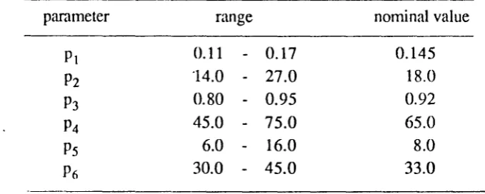
_n' Letp be redefined in R6such that,

reasonable ranges are listed in Table 3. Because most of the nominal values are located asymmetrically in the corresponding ranges, a beta distribution is used to describe the probability density for each parameter,

(8)

where

r(c

+

_{d )/( r(c) r(d) ) (bj - ai-c-<l(pj - al-1(b}j - pl-l, aj$ Pj $bj, b(c,d) = {

o

, otherwise,

with c > 0, andd>O. The distributions are assumed to be independent.

With this form for the probability density functions, the mode is taken to be the 'nominal value'. However, with only the modes and boundary values ofP, it is not possible to uniquely detennine the probability density. The two parameters, c andd, are relate9 to the mode by the following relation ( Johnson and Kotz, 1970),

mode( p )

=

a

+ (

b - a )( c - I )/(c

+

d - 2 ). (9) Reasonable shapes for the distributions being considered are obtained using the value of c=2.The values fordare obtained from the above equation and are listed in Table 4.

In the Monte Carlo simulation, random numbers, v, were generated, distributed according to the beta distribution, between 0 and 1, using the procedure of Yakowitz (1977). These values were then converted to values for parametersp,

Pi = ai

+ (

_{bi - ai ) v,} i=I,2, ...,6, (10) where Q_j and b_j are the minimum and the maximum values ofPi listed in Table 3. The

to solve the system equation. When an unrealistic solution is detected ( negative values of carbohydrate concentration in shoot or root), the parameter vector is discarded.

Since the magnitude of a regression coefficient in eqn (7) is dependent upon the units used for the independent variables, all the independent variables are standardized with respect to their means and standard deviations. Letm;and s; be the mean and standard

deviation of three hundred randomly generatedPi' The standardized variable z; is defined as

Zj = ( Pj -mj )/Sj , i=1,2, . . ., 6. (11) All of the statistical analyses to be reported are based on the variablezT

=(

z1- z2' z3' z4'

Z5' z6)' The response surface method ( Box, 1954) is used to approximate responses of

y with six independent variables

z

using the functional fonn

(12) It should be noted that the Yj are highly correlated. It is therefore appropriate to represent them by a single canonical variable ( Morrison, 1976). The first canonical variable, which will be labeledY4' explains about 94 percent of total variance of

y.

The

sensi ti vi ty coefficient of Y4with respect to a given parameter may then be used to represent

the system sensitivity. The response of Y4 to perturbation of parameter values is approximated by the functional fonn given in eqn (12). To estimate the values of parameters involved in eqn (12), the stepwise regression procedure in SAS was used, with significance level 0.05. In all cases, detennination coefticients (R2) of resulting equations

..

ZnT

=

(-0.1377, -0.5085, 0.8135, -0.2211, -0.0593, -0.4541).

From these notations, sensitivity coefficient of thei-th element ofy with respect to the j-th element ofp,Sjjcan be expressed as,

(13)

TIle calculated values ofsijare listed in Table 5:

RESULTS AND DISCUSSION

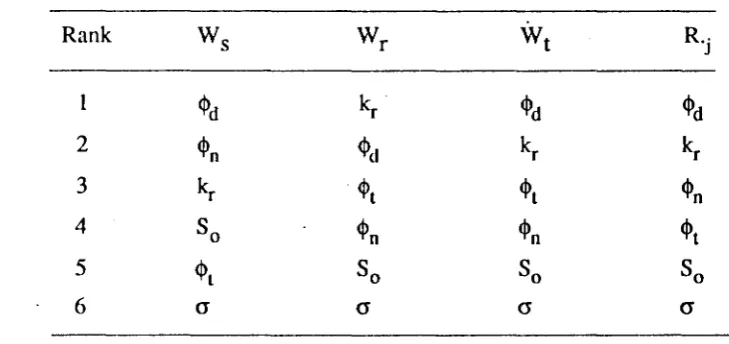
According to the magnitude of relative sensitivity coefficients approximated by 10 percent perturbation of parameter values (Table 2), the model is most sensitive to six parameters. These parameters are listed in Table 6 after ordering based on the magnitude

of the relative sensitivity coefficients. The parameters,

tl'd' tl'n'

tI'"

So' and a are the parameters related to carbohydrate concentration in the plant, while k_ris related to root growth. These results are reasonable because plant growth is dependent upon soluble carbohydrate concentration in the plant, and also upon nitrogen uptake rate which in turns depends on the root growth. Note that the system is also moderately sensitivetochanges in

Carney, 1981).

Both analyses are in agreement that

tP

_d' andk,are the parameters to which the system

is most sensitive. In fact,

tP

d is the most important parameter for controlling carbon input

from the environment, andk,is the parameter for controlling nitrogen input. Itis especially impollant to note that of the six parameters with a large relative sensitivity coefficient, three

ACKNOWLEDGEMENT

LITERATURE CITED

Box, G. E. P., 1954. The exploration and exploitation of response surface: some general considerations and examples. Biometrics

to,

16 - 60.

Burns,

J.

R., 1975. Error analysis of nonlinear simulations: application to world dynamics. IEEE Transactions on System, Man, and Cybernetics(5), 331 - 40.

Chatterjee, S., and Price, B., 1977. Regression Analysis by Example. John Wiley &

Sons, New York.

Draper, N. R., and Smith, fl., 1981. Appl(ed Regression Analysis. John Wiley & Sons, New York.

frank, P.M., 1978. Introduction to System Sensitivity Theory. Academic Press, New York.

Gardner, R. 11., O'Neill, R. V., Mankin, J. B., and Carney, J. H., 1981. A comparision of sensitivity analysis and error analysis based on a stream ecosystem model. Ecological Modelling 12, 173 - 90.

Huson, L. W., 1984. Definition and properties of a coefficient of sensitivity for mathematical models. Ibid. 21, ~49- 59.

Johnson, N. L., and Kotz, S., 1970. Continuous Univariate Distribution -2. Houghton Mifflin Company. Boston.

Lim, J. T., Wilkerson, G. G., Raper, C. D. Jr., and Gold, H.

J.,

1988. A dynamic growth model of vegetative soya bean plants: Model structure and behaviour under varying root temperature and nitrogen concentration. Journal of Experimental Botany 39, (accepted for publ.).

Morrison, D. F., 1976.Multivariate Statistical Methods. McGraw-Hill, New York. O'Neill, R. V., Gardner, R. H., and Mankin, J. B., 1980. Analysis of parameter error in

Steinhorst, R.

K,

Hunt, II. W., and lfaydock, K. P., 1978. Sensitivity analysis of the ELM model, pp. 231 - 56, In

Grassland simulation model,

ed. G. S. Innis. Springer Verlag, New York, NY.

Tomovic, R., and W. J. Karplus, 1963.

Sensitivity Analysis of Dynamic Systems.

McGraw-Hili, New York.

Table 1. List of parameters used in sensitivity analysis. index symbol 1

'"

2 _So

3

_rod 4

a

5

K

_p

6 n

7

K

_n

8

K

_c

9 k_s

10 k_r

11

11

12 G_r

13

cr

14 E

15

_<l>l 16 _<l>d 17 _<l>n 18

S

19

0

20 m description

Structural concentration of nitrogen in the plant Threshold storage CH₂0 concentration

End product inhibition coefficient Maximum photosynthetic rate

Michaelis-Menten constant in photosynthetic rate Power of the Hill equation

Mich\\elis-Menten constant of nitrogen uptake Michaelis-Menten constant of CI-LzO uptake Coefficient of shoot growth rate

Coefficient of root growth rate Leaf-weight leaf-area ratio Growth respiration coefficient Structural carbohydrate concentration Energy c,ost for nitrogen uptake

Net translocation coefficient of CH20 from shoot to root Net flow coefficient of CH₂0 from soluble CH₂0

pool to storage CH₂0 pool

Net flow coefficient of CH₂0 from storage CH₂0 pool to soluble CH₂0 pool

Net translocation coefficient of nitrogen from root to shoot

Table 2. R_{ij ,}and R'_j at 25-th day

j _{1 2 3}

R'j

1 0.0184 0.0223 0.0146 0.0552

2 2.2600 2.7692 1.6189 6.6481 . 3 -0.5941 -0.7253 -0.4292 1.7486

4 0.9028 1.1077 0.6440 2.6545

5 -0.2106 -0.2606 -0.1493 0.6205

6 0.2157 0.2641 0.1530 0.6328

Table 3. Estimated ranges of p and their nominal values

parameter range nominal value

PI

0.11

-

0.17

0.145

pz

14.0

-

27.0

18.0

P3

0.80

-

0.95

0.92

P4

45.0

-

75.0

65.0

Ps

6.0

-

16.0

8.0

Table 4. Parameter values of the beta distribution function of p.

variable c d

PI

2

1.5

P2

2

3.25

P3

2

1.25

P4

2

1.5

Ps

2

5.0

Table 5. The values of sensitivity coefficient (sij) by the response surface method.

j

1 2 . 3 4 5 6

Table 6. Rank ordering of the relative sensitjvity coefficients with the six parameters to which the model is most sensitive.

Rank _{W s Wr}

W

_t R._j

<Pd

~

<Pd <Pd

2 _{<Po <Pd kr kr}

3 _{kr <Pt <Pt <Po}

4 _{So <Po <Po <P}

t

5 _{<Pt So So So}