Speech Emotion Recognition with MPCA and Kernel Partial Least Squares Regression

Speech Emotion Recognition with MPCA and

Kernel Partial Least Squares Regression

Minghai Xin

School of Computer Science and Technology, Huaqiao University, Xiamen 361021 E-mail: [email protected]

Weiyi Gu

Research Centre for Learning Science, Southeast University, Nanjing, China, 210096 E-mail: [email protected]

Jinlong Wang

School of Computer Science and Technology, Huaqiao University, Xiamen 361021, E-mail: [email protected]

Abstract—Speech signal is one of the major means for communication which carries not only semantic, but personal information, such as genders and emotions. The researches about speech emotion have become more and more important to human-computer interaction. To this end, from speech, the long-term and short-term emotional features are extracted, the dimensionality of which is then reduced by virtue of the multi linear PCA algorithm. Finally, the kernel partial least squares regression is used for speech emotional recognition. The results show that in comparison with other current classifiers, the algorithm proposed herein can improve recognition rates by about 6% to 23%.

Index Terms—multi linear PCA; feature extraction; speech emotion recognition; kernel partial least squares regression

I. INTRODUCTION

Speech emotion recognition is one of the most promising modalities of affective computing besides expression recognition and whips up an increasing research interests around the world [1][2]. However, there are many difficulties in the field of speech emotion recognition. For example, unlike expression recognition, there is still no standard emotional speech database for researches. In addition, with different kinds of emotions, features and classifiers applied, it leads to various recognition rates ranging from 55% to 90% [3]. Ten Besch thought the actual recognition was approximately 60% [4].

Many researchers have proposed speech features which contain emotion information, such as energy, pitch frequency [5], formant frequency [6], Mel-Frequency Cepstrum Coefficients (MFCC) and its first derivative [7]. In general, two kinds of emotional features can be extracted from speech: long-term ones and short-term ones. However, due to less computation, faster classifying speed and higher recognition rates in many experiments, the long-term features are more frequently used. The dimension of speech features extracted is too

high, resulting in higher complexity of the computation. Increase in the number of the features would lead to not only greater calculation complexity, but also poorer recognition effect due to the redundancy information. Principal Component Analysis (PCA) [5] is a commonly used tool for dimension reduction in analyzing high dimensional data; Original PCA method is designed to firstly expand the training samples into a column or row of high-dimensional vector and then calculate the feature vectors of the training sample covariance matrix consisting projection matrix based on these vectors. Finally, the projection matrix changes a high-dimensional vector projection of the original training samples into a low one. However, vectorization process may destroy the object's underlying spatial structures and PCA runs into serious difficulties in analyzing functional data because of the “curse of dimensionality” (Bellman 1961). Hu proposed on the basis of the Multi linear PCA [8] that, the MPCA is a general extension of traditional linear methods, such as PCA or matrix SVD. The MPCA can obtain the variance of dimensionality reduction by directly using matrix or higher-order tensor, without transforming matrix or higher-order tensor into a vector for the PCA. Therefore, the above-mentioned problems can be overcome.

proposed herein can improve recognition rates by about 6% to 23%.

II.MULTI LINEAR PCAANALYSIS

A. Tensor

A tensor of orderNis defined as a multidimensional array or n-way array whose entries are accessed viaNindexes. A R∈ I I1× × ×2 ... IN is used an_Nthorder tensor,

where each element is denoted byai₁"i_N, and Rn is the Nvector space. Each dimension of a tensor is called nth-mode, where n refers to the nth index. Unfolding tensor A along the n-mode is denoted as

( n n N)

n I I I I

I× × × −× +× ×

∈ _R 1 " 1 1 "

n

A and An is a two dimensional

matrix. The n-mode product of a tensor A by a matrix_U ∈ _RIn×Jn, denoted byA U

n

× , is a tensor with entries as:

∑

= × _{− +} n n n N N n n n i i j ...i i ...i i j ...i i i

n U) a u

(A _{12 1 1 1} (1)

The scalar product of two tensors _A,b∈ _RI1×I2×...×IN is defined as:

1 2 1 2 1 2 N i i ...iN i i ...iN

i i i

< A,b >=

∑ ∑ ∑

... a b (2)

The Frobenius norm of A is defined as:

A = <A, A>.

According to standard multi linear algebra, any tensor A can be expressed as the

product 1 2

1 2

( ) ( ) (N)

N

A = S× U × U × ×... U . Where

1 2

1 2

( )T ( )T (N)T

N

S = A U× × U × ×... U , S is called as core

tensor that will be used for HOSVD and

) ...u u (u U (n) I (n) (n) (n) n 2 1

= is an orthogonalIn×In matrix.

B. Multi linear PCA Algorithm

Let’s take I1 I2 iN 1 2

m

{A ∈R ⊗R ⊗ ⊗... R ,m= , ,...,M} as a set of M tensor samples, the total scatter of these tensors is defined as

2 1 1 F M m m

A A A

M ψ

∑

= − = , where 1 1 M m m

A = A

M

∑

=

. The n-mode total scatter matrix

of these samples is then defined

as

1

M

(n) T

m(n) (n) m(n) (n)

m

S (A A )(A A )

=

=

∑

− − ,

where Am(n) is the n-mode unfolded matrix ofAm, A

is the mean tensor

1 1 M (n) _m(n) m A A M = =

∑

.

MPCA objective is the determination of the projection matrices{U∈RIn×Pn,n=1,...,N}that maximize the total

tensor scatter, ψy ,

( ) ( ) ( ) ( ) ( ) ( ) y U U U U U U P I N N n

n ,n ,...,N}

R U { _ψ , , , , , , max max argarg ~ " " 1 2 2

1

1 ₌

=

∈ ×

, where

2 1 M y m m F A A ψ =

=

∑

− , and

1 1 M m m A A m = =

∑

.

Accordingly, most of the variation observed in the original tensor objects can be captured, assuming that these variations are measured by the total tensor scatter.

With the MPCA method, the training speech features are rearranged into a 3D tensor as _{S ∈ R}I1×I2×I3, where

1

I is the emotion features of the speech, I2is the frame of the speech and I3 presents the number of speech used in the training phase. The multi linear PCA algorithm can be summarized as follows:

(1) Compute the mean matrix 3

1 3 1 I i i A A I ₌ =

∑

.

(2) Center the training tensorSˆ=[A1−A,A2 −A,...,AI3 −A]. (3) Unfold tensor into a matrix. For different modes, the unfolding matrices are different. The elements in the mode-n unfolding matrix are defined by

3 2 1ii i (imdex) (n) ) a

S

(ˆ = ,

where _⎥

⎦ ⎤ ⎢ ⎣ ⎡ Π − Π Π − = = − − == − = + = + = ∑

∑( )( I)( I)+ ( )( I)

, pm p

n m m p n p p n m p n m m

n i i

i index 1 1 1 1 1 1 1 1 3 1 1 .

(4) For a given mode-n, find the eigenvectors through covariance matrix T

) ( ) ( )

(n TˆnTˆn

C = , and

use [ , ,... ]

) (

)

(n x x xkn

X = 1 2 as the selected eigen vectors

which correspond to the largest k(n) _{eigenvectors.}

(5) Two types of feature selections processes can be performed: (a) using ( ) ( )

T

i n i n n

Y =(A -A)× X for different modes and (b) using ₁T ₂

i i ( )

Y =X (A - A)X .The first one provides k(1)× +I2 k(2)×I1features, whereas the second

one provides k(1)×k(2) features.

III.KERNEL PARTIAL LEAST SQUARES REGRESSION

As one of the most popular methods of metrology, PLSR has been proved to overtop traditional multi-variate statistical analysis methods in most linear cases. With the employment of a kernel, it can also work well in nonlinear problems.

A. Kernel Method

Kernel method is the common name of a series of advanced nonlinear data processing techniques, which all apply kernel mapping [9].

Let’s take

x

_i and

x

_j as the sample points in data space. Take

Φ

as the mapping function from data space to feature space. The kernel method is designed to realize inner-integral transformation between vectors:

(

xi,xj

)

→ K

(

xi,xj

)

=Φ

( ) ( )

xiΦٛ xj (3) Usually, nonlinear transformation Φ

()

ٛ

is very complicated while kernel function K(

C

,

C

), which is practically used, is relatively much simpler. Several common kernel functions are as follows:

(1) Linear kernel function. (special case)

(

)

j

T i j

i,x x x

x

(2) P-order kernel function.

(

)

[

( )

]

p

j T i j

i,x x x

x

K = ٛ +1 ₍₅₎

(3) Radial basis kernel function (RBF).

(

)

.

σ x x exp x , x

K _{i j} i j

⎟ ⎟ ⎟ ⎠ ⎞ ⎜

⎜ ⎜ ⎝

⎛ ₋

−

= ₂

2

(6)

(4) Multi-layer perception (MLP).

(

x,x

)

tanh

[

υ

( )

x x c

]

K _{i j = i}ٛ_{j +} (7)

Among these functions, radial basis function is the most widely used for its good learning ability.

B. Kernel-PLSR

The principle of Kernel-PLSR is to map the independent variable from original data space to new feature space by a special nonlinear transformation

Φ

and then to apply PLSR in the new feature space.

Just as shown in Figure 1, through the mapping by nonlinear transformation

Φ

, nonlinear classification problems could be turned to linear problems which could be solved by PLSR.

Figure 1. The transformation of feature space in

Kernel-PLSR

When the independent variable matrix is: p

* n p}

x , x , x {

X _{= 1 2 …} ,

and the dependent variable matrix is: q

* n q}

y , y , y {

Y _{= 1 2 …} ,

Φ

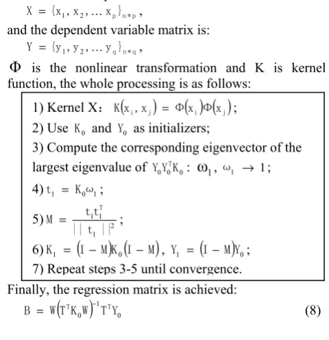
is the nonlinear transformation and K is kernel function, the whole processing is as follows:

Finally, the regression matrix is achieved:

(

)

0

1 0W TY

K T W

B ₌ T − T ₍₈₎

IV.FEATURE EXTRACTION

A. The Preprocessing of the Speech Signal

Speech signal preprocessing is a necessary pre-basic work, with its main steps as shown in Figure 2. The original speech samples after preprocessing can be used to further extract emotional features.

(1)Sampling and quantization

The original speech signal is a kind of analog signals, which will vary continuously over time. It is required to be converted into a digital signal in order for further processing by the computer. Sampling and quantization refers to the process where the analog signal is sampled according to the period and the amplitude is then quantified, as shown in Figure 2-2. The higher the sample frequency is, the shorter the sampling interval is and the more the information of the original signal is retained. When quantization is described by bit, N bits mean that the amplitude of the audio is represented with the 2n discrete order quantity. Therefore, a larger value of the

said bit will obtain a finer quantization result. However, the high fidelity also means the greater amount of the data, resulting in more time and resources consumed.. By full consideration of the research as stated herein, 8khz or 16khz sampling and 16bit quantification are generally applied for common emotion speech database.

As for Wav file in the library of current emotion speech, sampling has been completed via recording equipments such as microphones completed and included directly into one part of normalization.

(2)Normalization

As the recording volume varies from each person and will affect the role of the extracted feature parameters in the speech emotion recognition, the sampling value of the

1) Kernel X：K

(

x_i,x_j

)

₌ Φ

( ) ( )

x_iΦٛ x_{j ;}

2) Use K0 and Y0 as initializers;

3) Compute the corresponding eigenvector of the largest eigenvalue of Y0Y0K0

T _:

1

ω

, ω_{1 →} 1; 4)t1 = K0ω1;

5) ₂

1 1 1

|| t ||

t t M

T

= ;

6)K_{1 =}

(

I₋M

) (

K₀I₋M

)

, Y1 =

(

I−M

)

Y0; 7) Repeat steps 3-5 until convergence.

Sampling and

quantization Normalized Pre-emphasis

Windowed framing

Endpoint detection

speech signal is required to be normalized, in order to determine a more reasonable threshold. Normalization method generally used refers to the ratio of the sampling value and the maximum sample value:

( )

max

S n

S= _S (9)

(3)Pre-emphasis

Since the speech signal is effected by the glottal excitation and muzzle radiation, the power spectrum of its high-frequency end can reach about 800hz and will be decreased by 6dB / octave. The higher the frequency is, the smaller the amplitude will be. Therefore, the emphasis processing is required. The purpose of the pre-emphasis is to enhance the high frequency part and ensure the same signal-to-noise ratio for the entire frequency band in a bid to determine the spectrum by spectrum analysis or channel parameter analysis. In detail, to the pre-emphasis is a process where a digital signal passes through a high-pass filter and a is generally taken about 0.95.

( )

₁ 1_{,0.9 1.0}

H Z _{= − ⋅}a Z− _{≤ ≤}a ₍₁₀₎

(4)Windowed framing

The speech signal is a non-stationary random process, with time-varying characteristics. In a short range, the basic characteristics of the speech signal remain relatively stable, which can be seen as a quasi-steady-state process. So the speech signal is segmented to analyze its characteristic parameters. In order to achieve a smooth transition between frames overlapping segment is applied. The ratio between the frame shift length and the frame length is generally 0-0.5, depending on the specific circumstances:

Frame separation can be achieved by using mobile window of limited length to weight on the signal. The most common window functions in speech analysis are the rectangle window and Hamming window:

1) Rectangle window:

( )

n 1, 0_0, n N 1 n else ω =⎧⎨ ≤ ≤ −

=

⎩ (11)

2) Hamming window:

( )

0.54 0.46cos 2 1 ,0 1 0,

n _{n N}

n N

n else

π ω

⎧ ⎡ ⎤

− ≤ ≤ −

⎪ _{⎢ ⎥}

=⎨ ⎣ − ⎦

⎪ ₌ ⎩

(12)

The use of the window function ω

( )

n has the great influence on short-term analysis parameters of the speech signal. Rectangular window spectrum is smooth, but the high-frequency part of the signal is lost to make the detailed signal missing, which is opposite to Hamming window. Therefore extraction of the time-domain characteristic is usually provided with the rectangular window and extraction of the frequency-domain characteristic is usually offered with Hamming window. The choice of window length is usually combined with the pitch period of the speech signal. Generally speaking, a voice frame should contain 1-7 pitch period, so the frame length of 10ms-40ms is generally taken. The signal windowed can be represented as:

( )

( )

( )

w

S n =S n ⋅_ω n (13)

(5)Endpoint detection

Endpoint detection refers to the process where the start and end points of the speech is determined from a segment of signal which contains speech. It enables the extracted emotion characteristics to reflect information of the speech segment, rather than the noise dispersion. Therefore, it can help to improve the recognition rate and the calculation speed.

There are two major types of endpoint detection algorithms: threshold comparison method and model matching method. In this paper, the former method, as shown in Figure 3, is used to extract the characteristics of each frame and then compare such characteristics with the set threshold. Short-time energy, short-term average and short-term zero-crossing rate can be used as the endpoint detection extract characteristics.

(a) The short-term energy sequence of a speech signal, where TH corresponds to a threshold value (b) The short-term energy sequence of the speech signal after endpoint detection

B. Speech Emotion Features Extraction Approach One of the important tasks at this stage after pre- processing is to extract features. It is important in speech emotion recognition to find out proper features, so as to best present different emotions. Due to less computation, faster classifying speed and better recognition rates in many experiments, our goal is to extract the long-term features rather than short-term features in our experiment. First of all, the raw contours of energy is extracted on the basis of long –term features; pitch (F0) and formants (F1, F2, F3) are well-known for their capability to carry large emotional information. In order to do this, 20 ms frames of the speech signal are analyzed every 10ms, by using a Hamming window function. Logarithmic energy within a frame is used to calculate the energy contour, and the pitch contour is achieved by use of a modified cepstrum-based algorithm [12]. The first formants estimation is based on resonance frequencies in the LPC-spectrum with the order 20. The unvoiced sections in energy, pitch and formants contours are eliminated to get more independence of the spoken content and achieve better recognition results. After the adjusted contours of energy, pitch (F0) and formants (F1, F2, and F3) are extracted, the first and the second order derivatives of which are then calculated. Then, statistics of each contour are completed, including mean, maximum, minimum, median, range, variance and interquartile. These statistics form part of final features.

Additionally, speed, durations, v/uv and E250 are also calculated as features. The former three are all based on intensity, whereas E250, namely energy below 250Hz, is achieved by calculating the FFT spectrum for each frame.

The whole long-term feature list includes: [1]. Speed (mean syllables per second). [2]. Energy below 250 Hz (E250).

[3-16]. Duration of voiced and unvoiced parts: max, min, mean, median, range, variance and interquartile.

[17]. v/uv (ratio of the total duration of voiced parts to the one of unvoiced parts).

[18-38]. Pitch (F0) and its first 2 orders derivatives: max, min, mean, median, range, variance and interquartile.

[39-80]. The first three formants (F1, F2 and F3) and their first 2 orders derivatives: max, min, mean, median, range, variance and interquartile.

[81-101]. Energy and its first 2 orders derivatives: max, min, mean, median, range, variance and interquartile.

All the above features will be normalized to produce the same weight in classification.

V SPEECH EMOTION FEATURE EXTRACTION AND

AUTOMATIC CLASSIFICATION

MPCA is a multi linear subspace learning method that extracts features directly from multi-dimensional objects. MPCA receives the set of emotional samples of the same dimensions as input for feature extraction. The resultant output of the MPCA is the dimensionally reduced feature projection matrix of speech signals.

Kernel-PLSR is used for classification in this experiment. Radial basis function is chosen as the kernel function for its good learning ability. But it is not easy to decide the value of the parameter

σ

of RBF, which is very sensitive to the performance of classification. [13] proposed an effect method for determining

σ

. Let

2 2 i med

σ

=

k d

(14)

where

k

_i

∈

{

1

₈

,

1

₄

,

1

₂

,1, 2, 4

}

, and

d

_med is the median distance among samples of different emotions. Try different

k

_i to find the one which leads to best recognition results. This way to pick the optimal

σ

will be applied in our experiment.

To compare with the performance of Kernel-PLSR, principle component analysis (PCA), linear discrimination analysis (LDA), k-nearest neighbor (kNN), Gaussian mixture model (GMM) and PLSR will also be studied. In GMM, up to four mixtures have been used and each emotion is modeled by one GMM. The maximum likelihood model will be considered as the recognized emotion for each test sample.

VI.EXPERIMENTAL RESULTS

The database used herein is Berlin emotional speech database [12]. In this database, ten actors (5 female and 5 male) simulated seven emotions (anger, disgust, fear, joy, sadness, boredom and neutral), producing 10 German utterances (5 short and 5 longer sentences) which could be used in daily communication and are interpretable in all applied emotions. The database is recorded in 16 bit, 16 kHz under studio noise conditions.

In this paper, five typical emotions of them are selected for study: anger, fear, joy, sadness, boredom. In order not to favor one emotion over the others, only fifty-three samples are randomly selected from each emotion. As a general mean of evaluation, thirteen-folder cross validation is used.

In this paper, 101 global statistic features are extracted from Berlin emotional speech database, and five classifiers are used to distinguish five emotions.

Multi linear PCA is used for classification in this experiment. To compare with the performance of MPCA-KPLSR, principle component analysis (PCA), linear discrimination analysis (LDA), k-nearest neighbor (kNN), Gaussian mixture model (GMM) and PLSR will also be studied. In GMM, up to four mixtures have been used and each emotion is modeled by one GMM [13]. The maximum likelihood model will be considered as the recognized emotion for each test sample.

Table 1 shows the recognition rates by use of multi linear PCA and the average recognition rate is 78.08%.

Table 2 shows the recognition rates by use of PCA and nearest neighbor classifier.

Table 3 shows the recognition rates by use of LDA and nearest neighbor classifier.

Table 5 shows the recognition rates by use of PLSR classifier.

In these tables, fea is the abbreviation for fear, sad for sadness, ang for anger and bor for boredom.

TABLE 1.

CONFUSION MATRIX OF THE MPCA-KPLSR ALGORITHM WITH

78.08% MEAN RECOGNITION RATE

Labeled emotion

Recognized emotion (%)

fea joy sad ang bor

fea 73.08 9.62 5.77 9.62 1.92

joy 17.31 59.62 0 21.15 1.92

sad 3.85 0 90.38 0 5.77

ang 3.85 15.38 0 80.77 0

bor 0 5.77 5.77 1.92 86.54

TABLE 2.

CONFUSION MATRIX OF THE PCA+1NN CLASSIFIER WITH 56.54%

MEAN RECOGNITION RATE

Labeled emotion

Recognized emotion (%)

fea joy sad ang bor

fea 36.54 28.85 7.69 23.08 3.85

joy 15.38 44.23 0 36.54 3.85

sad 7.69 0 78.85 0 13.46

ang 13.46 38.46 0 46.15 1.92

bor 3.85 5.77 11.54 1.92 76.92

TABLE 3.

CONFUSION MATRIX OF THE LDA+1NN CLASSIFIER WITH 56.92% MEAN RECOGNITION RATE

Labeled

emotion Recognized emotion (%) fea joy sad ang bor

fea 36.54 28.85 3.85 13.46 17.31

joy 25.00 42.31 1.92 25.00 5.77

sad 0 1.92 73.08 1.92 23.08

ang 5.77 32.69 1.92 57.69 1.92

bor 3.85 7.69 13.46 0 75.00

Hydroelectric power plants generally require the creation of a large artificial lake. Evaporation from this lake is higher than that from a river due to the larger surface area exposed to the elements, resulting in much higher water consumption. The process of driving water through the turbine and tunnels or pipes also briefly removes this water from the natural environment, creating water withdrawal. The impact of this withdrawal on wildlife varies greatly depending on the design of the power plant.

TABLE 4.

CONFUSION MATRIX OF THE GMM CLASSIFIER WITH 62.31% MEAN RECOGNITION RATE

Labeled emotion

Recognized emotion (%)

fea joy sad ang bor

fea 42.31 30.77 9.62 13.46 3.85

joy 13.46 57.69 0 25.00 3.85

sad 3.85 0 86.54 0 9.62

ang 21.15 34.62 0 44.23 0

bor 0 3.85 13.46 1.92 80.77

TABLE 5.

CONFUSION MATRIX OF THE PLSR CLASSIFIER WITH 72.69% MEAN RECOGNITION RATE

Labeled emotion

Recognized emotion (%)

fea joy sad ang bor

fea 75.00 17.31 5.77 1.92 0

joy 9.62 51.92 0 28.85 9.62

sad 5.77 1.92 82.69 1.92 7.69

ang 0 25.00 1.92 67.31 5.77

bor 0 3.85 5.77 3.85 86.54

The following table 6 gives an overview of classifiers comparison and the accuracy data stands for the average recognition rate of five emotions under each classifier. Obviously, this multi linear PCA gains optimal results.

TABLE 6.

COMPARISON OF FIVE CLASSIFIERS

classifier Accuracy (%)

PCA + 1NN 56.54

LDA + 1NN 56.92

GMM 62.31 PLSR 72.69

MPCA-KPLSR 78.08

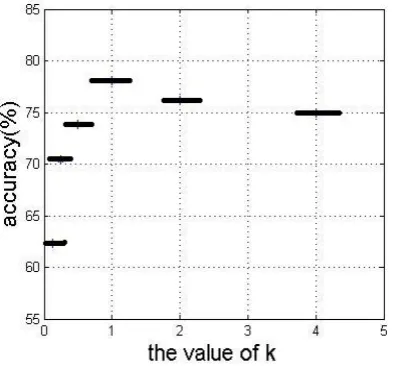
Figure 4 demonstrates the influence of the parameter value of the RBF kernel. The horizontal axis stands for

i

k

referring to equation 7, while the vertical axis stands for the mean recognition rates of five emotions using kernel-PLSR with different parameter k. And

d

2_med here

has been worked out as 5.8716. It can be seen in this figure, the highest recognition rate 78.08% is gained

when k=1.

Figure 4. Influence of the parameter value of the RBF kernel

VII.CONCLUSION

REFERENCES

[1] R.Cowie, “Emotion Recognition in Human-Computer Interaction”, IEEE Signal Processing Magazine, vol.18, No.1, pp.32-80, Jan.2001.

[2] M. Pantic, L. Rothkrantz, “Toward an Affect-Sensitive Multimodal Human-Computer Interaction”, Proceedings of the IEEE, Vol.91, pp. 1370-1390, Sep. 2003.

[3] Li Zhao, Speech Signal Processing, Beijing: Mechanical Industry Press, 2003.

[4] Jiqing Han, Yanqiu Shao, “Research Progress of Emotion Processing Based on Speech Signal”, Voice Technology, Num: 1002-8684(2006)05-0058-05.

[5] D. Ververidis, C. Kotropoulos, and I. Pitas, “Automatic emotional speech classification”, in Proc. 2004 IEEE Int. Conf. Acoustics, Speech and Signal Processing, vol. 1, pp. 593-596, Montreal, May 2004.

[6] Xiao, Z., E. Dellandrea, Dou W.,Chen L., “Features Extraction and Selection for Emotional Speech Classification”. 2005 IEEE Conference on Advanced Video and Signal Based Surveillance (AVSS), pp.411-416, Sept 2005.

[7] S. Wold, H. Martens, H. Wold, “The Multivariate Calibration Problem in Chemistry Solved by the PLS Method”, Ruhe A, Kågström B(Eds), Proc. Conf. Matrix Pencils, Lectures Notes in Mathematics, Heidelberg: Springer-Verlag, 1983.

Haiping Lu, K.N. Plataniotis, et al, MPCA: Multilinear Principal Component Analysis of Tensor Objects[J], IEEE Transactions on Neural Networks, January, Vol.19,No.1, pp.18-39, 2008

[8] R. Rosipal, L. Trejo, “Kernel Partial Least Squares Regression in Reproducing Kernel Hibert Space”, Journal of Machine Learning Research, 2001, 2:97-123.

[9] K.R. Muller, S. Mika, G. Ratsch, “An Introduction to Kernel-Based Learning Algorithms”, IEEE Transactions on Neural Network, 2001, 12(2): 180-201.

[10]Xuecheng Jin, Ling Xie, Zengfu Wang, “A Modified Cepstrum-Based Algorithm for Fundamental Frequency Estimation Using Dynamic Programming”, Technical Acoustics, Vol.27, No.1, Feb., 2008.

[11]Xiang Zhang, Xiaoling Xiao, Guangyou Xu, “A New Method for Determining the Parameter of Gaussian Kernel”, Computer Engineering, Vol.33, No.12, June,2008 [12] http://www.expressive-speech.net/, Berlin Emotional

Speech Databases.

[13]T.-L. Pao, Y.-T. Chen, J.-H. Yeh, P.-J. Li, “Mandarin Emotional Speech Recognition Based on SVM and NN”, Proceedings of the 18th International Conference on Pattern Recognition (ICPR 06), vol. 1, pp. 1096-1100, September 2006.

Minghai Xin received the M.S. degrees from Huaqiao