ABSTRACT
SHEN, WEINING. Adaptive Bayesian Function Estimation. (Under the direction of Subhashis Ghosal.)
This dissertation focuses on developing some new Bayesian methodologies for function es-timation and studying their theoretical properties. In particular, we investigate conditions under which such methods achieve the optimal posterior rate of convergence even when the smooth-ness of the underlying function is unknown. Some examples of functions of interest include density function, conditional density function, regression function, and classification function. Although several nonparametric Bayesian models have been developed for many applications, their theoretical properties, such as large-sample convergence properties are often not fully understood. Part of the dissertation focuses on exploring the posterior convergence rates of certain nonparametric Bayesian procedures. We establish rate-adaptive Bayesian procedures in the sense that the optimal minimax rate of estimation can be achieved by using one single prior for the entire smoothness class that the underlying true function belongs to. Such results can be viewed as frequentist large-sample justification, which suggests that by carefully selecting priors, the posterior distribution of the estimator concentrates around the truth at an optimal rate.
In Chapter 2, we consider a multivariate density estimation problem. We show that rate-adaptive Bayesian procedures can be obtained using Dirichlet mixtures of multivariate normal kernels with a prior distribution on the kernels covariance matrix parameter. Locally H¨older smoothness classes and their anisotropic extensions are considered. Our study involves sev-eral technical novelties, including a sharp approximation of finitely differentiable multivariate densities by normal mixtures and a new sieve on the space of such densities.
estimation problems. The prior is constructed through distributions on the number of basis functions and the associated coefficients. We derive a general result on the construction of an appropriate sieve and obtain adaptive posterior contraction rates. This general result is applied on several statistical problems such as signal processing, density estimation, nonparametric regression, classification, spectral density estimation, functional regression etc. The random series prior can be viewed as an alternative to the commonly used Gaussian process prior, but can be analyzed by relatively simpler techniques and in many cases allows a simpler approach to computation without using Markov chain Monte-Carlo (MCMC) methods.
In Chapter 4, we extend the random series prior to a multivariate setting. In particular, we consider a density regression problem (i.e., estimation of a conditional density function) in a high-dimensional situation, in which the number of covariates is possibly much larger than the sample size. We develop a MCMC-free computing technique to calculate the poste-rior moments of the conditional density. Adaptive convergence rate is obtained under sparsity conditions that adapts to both the smoothness level and the actual number of covariates that influence the conditional density.
© Copyright 2013 by Weining Shen
Adaptive Bayesian Function Estimation
by Weining Shen
A dissertation submitted to the Graduate Faculty of North Carolina State University
in partial fulfillment of the requirements for the Degree of
Doctor of Philosophy
Statistics
Raleigh, North Carolina 2013
APPROVED BY:
Eric Laber Surya T. Tokdar
Huixia Wang Subhashis Ghosal
DEDICATION
BIOGRAPHY
ACKNOWLEDGEMENTS
To begin with, I would like to express my deepest gratitude to my advisor Dr. Subhashis Ghosal for his generous support throughout my graduate studies, for his patience, motivation, enthusi-asm, and immense knowledge. His tremendous work ethics and passion towards academics set me a good example to stay motivated and persistent.
I would also like to extend my appreciation to my committee members, Dr. Eric Laber, Dr. Surya T. Tokdar and Dr. Huixia Wang for their constant encouragement and wonderful advices. In particular, Chapter 2 is based on a joint work with Dr. Tokdar. It has been a great privilege to work with them. Thanks to Dr. Peter Bloomfield, Dr. Howard D. Bondell, Dr. Dennis D. Boos, Dr. David A. Dickey, Dr. Sujit K. Ghosh, Dr. Lexin Li, Dr. Wenbin Lu, Dr. John F. Monahan, Dr. Jason A. Osborne, Dr. Brian J. Reich, Dr. Shan Suthaharan, Dr. Anastasios Tsiatis, Dr. Daowen Zhang and Dr. Hao Zhang for teaching me so many wonderful courses and giving me inspiring comments in my research.
Thanks to my fellow students and friends at NCSU. Life will be much harder without your accompany. To Dehan Kong, Zhuo Yan, Guolin Zhao, Juan Fang, Shu Wang, Jingwen Zhou, Jiangdian Wang, Jialong Cheng, Xiang Zhang, Xianyang Zhang and Gongjun Xu, your friendship has enriched my life journey.
I am grateful to Regeneron Pharmaceuticals Inc and First Analytics for offering me intern-ship opportunities. Sincere thanks to my former colleagues Haobo Ren, Richard Wu, Yuhwen Soo, Liming Liu, Jenny, Yunling Du, Mike Thompson and Ken Anderson for sharing their working and life experiences with me.
TABLE OF CONTENTS
LIST OF TABLES . . . ix
LIST OF FIGURES . . . x
Chapter 1 Introduction . . . 1
1.1 Overview of nonparametric Bayesian . . . 1
1.2 Common priors . . . 3
1.2.1 Dirichlet process . . . 3
1.2.2 Dirichlet process mixture . . . 4
1.2.3 Gaussian process . . . 5
1.2.4 Tail-free process . . . 7
1.2.5 Basis expansion . . . 9
1.3 Asymptotics . . . 10
1.4 Adaptation . . . 14
1.5 Notations . . . 15
1.6 Outline . . . 18
Chapter 2 Multivariate density estimation using Dirichlet mixture of normal prior 19 2.1 Introduction . . . 19
2.2 Posterior Convergence Rates for Dirichlet Mixtures . . . 21
2.2.1 Dirichlet process mixture of multivariate normals prior . . . 21
2.2.2 Locally H¨older classes . . . 24
2.2.3 Convergence rates results . . . 26
2.3 Prior thickness results . . . 28
2.4 Sieve construction . . . 38
2.5 Supplementary results . . . 43
2.6 Proof of Theorems 3 and 4 . . . 49
2.7 Anisotropic H¨older functions . . . 50
Chapter 3 Univariate function estimation using random series prior . . . 54
3.1 Introduction . . . 54
3.2 General results . . . 58
3.2.1 Main theorem . . . 58
3.2.2 Posterior convergence rates . . . 62
3.2.3 Approximation ability of B-splines . . . 69
3.3 Gaussian white noise model . . . 71
3.4 Density estimation . . . 73
3.4.1 Density on the unit interval . . . 73
3.4.3 Density estimation using B-splines . . . 76
3.5 Whittle estimation of spectral density . . . 78
3.5.1 Posterior convergence rates . . . 78
3.5.2 Computation using B-splines . . . 80
3.6 Nonparametric regression with Gaussian errors . . . 81
3.6.1 Posterior convergence rates . . . 81
3.6.2 MCMC-free Computation . . . 84
3.7 Nonparametric binary regression . . . 85
3.7.1 Posterior convergence rates . . . 85
3.7.2 Computation using B-splines . . . 87
3.8 Nonparametric Poisson regression . . . 89
3.8.1 Posterior convergence rates . . . 89
3.8.2 Computation using B-splines . . . 90
3.9 Functional regression model . . . 91
3.9.1 Functional covariates . . . 92
3.9.2 Functional responses . . . 93
3.9.3 MCMC-free computation . . . 94
3.10 Extension to other function spaces . . . 94
3.11 Numerical results . . . 97
3.11.1 Density estimation . . . 97
3.11.2 Binary regression . . . 98
3.12 Conclusion . . . 101
Chapter 4 Density regression for high-dimensional data . . . 103
4.1 Introduction . . . 103
4.2 Bayesian density regression . . . 106
4.2.1 Prior . . . 106
4.3 Posterior convergence rates . . . 108
4.3.1 MCMC-free Computation . . . 113
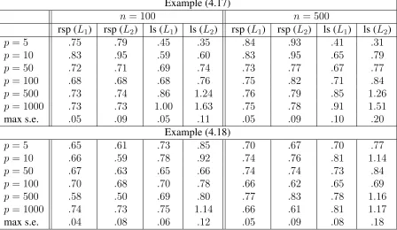
4.4 Numerical results . . . 115
4.4.1 Computing algorithm . . . 115
4.4.2 Simulation studies . . . 116
Chapter 5 Adaptive derivative estimation . . . 118
5.1 Introduction . . . 118
5.2 Prior . . . 119
5.2.1 Dirichlet mixture prior . . . 119
5.2.2 Finite mixture prior . . . 120
5.2.3 Random series prior . . . 121
5.3 Posterior convergence rate . . . 122
5.3.2 Approximation results . . . 127
5.3.3 Proof of Theorem 21 . . . 130
REFERENCES. . . 131
APPENDIX . . . 140
Appendix A Introduction to B-splines . . . 141
A.1 Univariate B-splines . . . 141
LIST OF TABLES
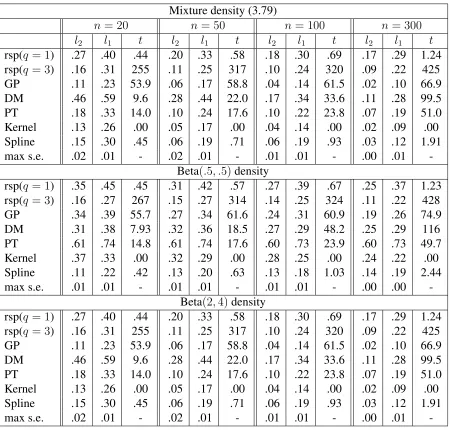
Table 3.1 Density estimation examples . . . 99
Table 3.2 Binary regression examples (3.80)–(3.82). . . 100
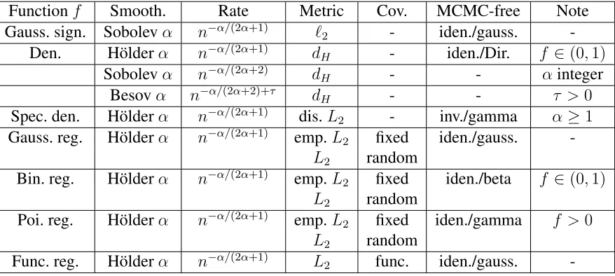
Table 3.3 Summary of convergence rates and MCMC-free computation . . . 102
LIST OF FIGURES
Chapter 1
Introduction
1.1
Overview of nonparametric Bayesian
Nonparametric models are widely used in many areas of statistic studies (Wasserman, 2006). Compared with parametric models, which assume that the distributions are based on only a few parameters in a particular functional form, nonparametric models are more flexible in the sense of having a much larger parameter space and relying upon fewer assumptions. Nonparamet-ric inference covers a wide range of different topics such as constructing test procedures that are “distribution-free” at least in the asymptotic sense, estimating functions without any para-metric assumptions, computation techniques such as bootstrap etc. In the thesis, we focus on function estimation problems. Some examples of functions of interest include density function, cumulative distribution function, quantile function, regression function, classification function, spectral density, hazard rate function and so on.
there are many attractive properties of the Bayesian approach that makes it quite popular. For example, the inference is straightforward once the posterior distribution is obtained. It is simple to obtain and interpret predictions and intervals estimates. With the development of innovative computational algorithms such as Monte-Carlo Markov chain (MCMC) and variational meth-ods, Laplace approximation etc. and the availability of powerful computational resources, most Bayesian methods can now be implemented within a reasonable time.
1.2
Common priors
1.2.1
Dirichlet process
We first discuss the Dirichlet process (DP), one of the most classic and popular choices of prior in the infinite-dimensional world. The concept was first introduced by Ferguson (1973). The formal definition is given below
Definition 1. A random measureP is called a Dirichlet process on a measurable spaceXwith parameter αif for every finite measurable partition {B1, . . . , Bk}ofX, the joint distribution
of(P(B1), . . . , P(Bk))follows a Dirichlet distribution with parameters(α(B1), . . . , α(Bk)). We denote this Dirichlet process byDP(α), whereαis a finite measure onX.
Dirichlet processes have many nice properties. Conceptually, it can be viewed as an infinite-dimensional generalization of the Dirichlet distribution. The Dirichlet process is conjugate for independent and identically distributed (i.i.d.) observations, which makes posterior compu-tations straightforward. Moreover, it has an interesting stick-breaking representation (Sethu-raman, 1994), which leads to some useful MCMC sampling algorithms for priors based on Dirichlet mixture processes. This result turns out to be very helpful in our study in Chapter 2. There are many other interesting properties as listed below.
• (Stick-breaking representation) A Dirichlet processP ∼DP(α)can be represented as
P =
∞
∑
i=1
πhδZh, πh =Vh∏ j<h
(1−Vj), Vi ∼Beta(1,|α|), Zh ∼α,¯ (1.1)
where|α|=α(X)andα¯ =α/|α|.
posterior distribution ofP givenXisDα+∑n
i=1δXi, whereδx is a point mass probability
measure on a pointx.
• (Discreteness) An interesting property of a DP is that sampling distributions from it are always discrete, even when the base measure is continuous.
1.2.2
Dirichlet process mixture
When estimating a continuous density function, a Dirichlet process prior is not appropriate because it is discrete. Hence a Dirichlet process mixture is usually used (Ferguson, 1983; Lo, 1984) by convoluting a Dirichlet process with a probability density kernel functionΨ parame-terized byθas follows:
Xi ∼ pF(x) =
∫
Ψ(x, θ)dF(θ), i= 1, . . . , n; F ∼DP(α). (1.2)
By introducing latent variablesθ1, . . . , θn, the model can be equivalently written as
Xi|θi ∼Ψ(x, θi), θi|F
i.i.d.
∼ F, i= 1, . . . , n; F ∼DP(α). (1.3)
Then by the conjugacy property of a Dirichlet process, we get the posterior ofF givenθ1, . . . , θn asF|θ1, . . . , θn∼DP(α+
∑n
i=1δθi). Hence we obtain the posterior expectation of the density
as
E{pF(x)|θ1, . . . , θn}=
α(R)
α(R) +n
∫
Ψ(x, θ)dG(θ) + 1
n n
∑
i=1
Ψ(x, θi).
Therefore, many MCMC computation algorithms have been developed including Gibbs sam-pling based on the P´olya urn schemes (Escobar and West, 1995; MacEachern and M¨uller, 1998), methods based on truncation of a Dirichlet process (Ishwaran and James, 2001), retro-spective sampling methods (Papaspiliopoulos and Robers, 2008), and slice sampling methods (Walker, 2007).
1.2.3
Gaussian process
Another popular class of priors are constructed via Gaussian processes (Leonard, 1978; Lenk, 1988, 1991). A Gaussian process (GP) can be viewed as an infinite-dimensional generalization of a Gaussian distribution. The formal definition is as follows.
Definition 2. A stochastic process{Xt, t ∈T}is called a Gaussian process if for every finite
index set(t1, . . . , tk)∈T, the joint distribution of(Xt1, . . . , Xtk)is Gaussian.
The distribution of a GP onRT is uniquely determined by its mean functionµ(t) = E(Xt) and covariance kernelK(s, t) = E(XsXt). We give some examples here for illustration.
Example 1. Brownian motion
A Brownian motion Bt is a continuous stochastic process that was first used to model the random moving of a particle in the fluid. A standard Brownian motion on the positive line can be viewed as a Gaussian process withµ(t) = 0andK(s, t) = min(s, t).
Example 2. Fractional Brownian motion
Fractional Brownian motions generalize a standard Brownian motion without independent in-crements. Again, it is a Gaussian process with
whereα ∈ (0,1)is called a Hurst parameter, which controls the correlation of increments of the process. When choosingα= 1/2, we obtain a Brownian motion.
Example 3. Integrated Brownian motion
In order to smooth a Brownian motion, we take its integral and obtain integrated Brownian motions as a result. For example, the smoothness level of ak-fold integrated Brownian motion isk+ 1/2. Again, such process is a Gaussian process with
µ(t) = 0, K(s, t) =
∫ min(s,t)
0
(s−u)k(t−u)k (k!)2 du.
Example 4. Gaussian process with a squared exponential kernel
Another example of the kernel is squared exponential function K(s, t) = exp{−c(s−t)2}, wherecis a hyper-parameter. This kernel is stationary in the sense that it only depends on the difference of the inputs (s −t). Such a kernel has been widely used in the kernel machine learning literature. The resulting Gaussian process has infinitely smooth sample paths.
Example 5. Finite series expansion
Considerki.i.d random variablesZ1, . . . , Zk ∼N(0,1)and some real-valued functionsa1, . . . , ak. Then the stochastic processWt=
∑k
i=1ai(t)Zi is a Gaussian process with
µ(t) = 0, K(s, t) =
k
∑
i=1
ai(s)ai(t).
(2007) and many others. Theoretical properties of a GP can be elegantly expressed in terms of on its reproducing kernel Hilbert space (RKHS). van der Vaart and van Zanten (2009) ap-plied a random rescaling technique on GP priors and showed that such procedures have nice asymptotic properties such as Bayesian adaptation etc.
1.2.4
Tail-free process
A tail-free process is another popular class of processes to construct priors for absolutely con-tinuous probability distributions under certain conditions. Dirichlet process also belongs to this class. Tail-free process priors are constructed based on partitioning a setX⊆ R. Without loss of generality, we consider a binary partition as an example. Let {Γk : k = 1,2, . . .} denote nested partitions ofX. For example,
Γ1 = (B0, B1);B0 =B00∪B01;B1 =B10∪B11,
Γ2 = (B00, B01, B10, B11);Bij =Bij0∪Bij1, i = 0,1, j= 0,1,
Γ3 = (B000, B001, B010, B011, B100, B101, B110, B111).
In other words, everyΓk+1is a refinement of its previous partitionΓksatisfying the relationship Bs = Bs0 ∪Bs1, where s is some{0,1} sequence. By defining random variables Vs as the
probability on a set Bs and assume that variables defined in different Γk are independent to each other, we may obtain a tail-free random probability measure defined on X. DefineΓ as the collection ofΓ1, . . . ,Γk. A formal definition is as follows:
Definition 3. A random probability measureP onXis tail-free with respect to(Γ,X)if there exist nonnegative random variables{Vs:s∈ {0,1}k, k≥1}defined onBssuch that
different values ofk.
(ii) P(Bs) = ∏k
i=1Vs1···si for everys∈ {0,1}
k,k≥1.
Obviously, this definition can be extended beyond binary partitions. It is also possible to consider varying number of subsets in different partition levels. One of the nicest properties of tail-free process prior is its conjugacy structure. Here we list a few properties, their proofs can be found in Freedman (1963, 1965).
• (Conjugacy) Given i.i.d observationsX1, . . . , Xn|P ∼ P, in whichP is a tail-free prior with respect to(Γ,X), then the posterior is another tail-free process with respect to the same partition(Γ,X).
• (Continuous or discrete) Given a tail-free processP with respect to(Γ,X). Suppose there is a measureλ such thatλ(B) > 0for every B ∈ H. ThenP is absolutely continuous with respect toλwith probability zero or one. As a result,P is discrete with probability zero or one.
• (Transformation) The tail-free property is preserved under monotonic transformations. • (Mixture) The tail-free property is not preserved under mixture operation.
Besides Dirichlet process, another popular tail-free process is called Polya tree process Blackwell and MacQueen (1973); Ferguson (1974). A Polya tree process is defined through binary partitions as follows:
Unlike the Dirichlet process, a Polya tree process gives rise to continuous distributions. It has been used in nonparametric Bayesian density estimation (Lavine, 1992, 1994). The Polya tree family has a conjugacy property that makes the updating of the posterior distribution sim-ple.
Theorem 1. Given i.i.d observationsX1, . . . , Xn|P ∼ P and P ∼ PT(Γ,α), the posterior
process is another Polya tree PT(Γ,α∗), where α∗s = αs +
∑n
i=11l(Xi ∈ Bs) for every
s∈ {0,1}k,k ≥1.
However, one limitation of a Polya tree process prior is its dependence on the partition sets. Also, there might be discontinuity issues at the boundary of partition sets, which is not desired in situations such as density estimation. To address this issue, mixtures of Polya trees have been considered in Hanson and Johnson (2002).
1.2.5
Basis expansion
In function estimation problems, it is common to expand the unknown function f by pre-specified basis functions{ξj}:f =∑Jj=1θjξjor through some link function:f = Ψ(∑Jj=1θjξj). Then by assigning prior distributions on J and relevant coefficient θj’s, we obtain a prior on the functionf. Some commonly used bases include polynomials, splines and wavelets. In some situations, in order to induce a valid prior on the function of interest, it may be necessary to consider a specific link function or to put restrictions on the coefficientsθj. For example, for density estimation problems, in order to make f nonnegative and integrate to one, we may choose splines as basis, restrict all coefficients to be nonnegative and then rescale it as follows
f(x) =
∑∞
j=Jθjξj(x)
∫ ∑∞
This idea applies for some functions with complex forms as well. For example, in Chapter 3.9, we consider a functional regression model where each coefficient is now a functional of time. In Chapter 4, the function we are interested in is a conditional density under a high-dimensional setting.
1.3
Asymptotics
In this section, we discuss the asymptotic properties of Bayesian procedures in a frequentist sense. Denotef as the function of interest. Intuitively, one would expect the posterior concen-trate around the true function f0 if there are infinitely many data available. This property is called posterior consistency and is mathematically defined as
Π(d(f, f0)> ϵ|X1, . . . , Xn)→0,inPfn0-probability. (1.4)
If the posterior distribution is available in an explicit form, then posterior consistency may be obtained by applying certain moment inequalities such as Chebyshev’s inequality. This is the case in some Bayesian survival analysis problems and other places where conjugacy structure is available. However, in most applications this approach is not feasible. A more useful result was established by Schwartz (1965) for dominated families. The theory gives two sufficient condi-tions for consistency. First, withf0being the true function, there should exist a strictly unbiased test forf =f0against complement of the neighborhood off0. This ensures that the type I and type II error probabilities are going to zero exponentially fast. Secondly, the prior should have a positive probability in any neighborhood of the true function in a Kullback-Leibler (KL) diver-gence sense. Here the KL diverdiver-gence between two probability densitiespandq(with respect to a dominating measure ν) is defined asK(p, q) = ∫ plog(p/q)dν. The second condition is crucial and sometimes is referred to as the Kullback-Leibler property. The KL divergence can be stronger than the natural distance on the parametric space. Unfortunately, Schwartz’s test-ing condition does not hold for many nonparametric problems for stronger topologies unless the parameter space is compact, which is a very strict requirement. A refined result was pro-posed by Ghosal et al. (1999) using a technique involving sieves. A sieve is defined as a big subset of the parameter space. They showed that by carefully choosing a sieve and then apply-ing Schwartz’s techniques on the sieve, posterior consistency can be obtained by boundapply-ing the prior probability of the complement of the sieve and the entropy number of the sieve. This idea was initially used by Barron et al. (1999) under stronger conditions using bracketing entropy.
Besides consistency, convergence rate is another issue of extreme importance in asymp-totics. It measures the speed of the convergence of posteriorf given the dataX1, . . . , Xnto the true valuef0under some metricd. A sequenceϵn →0is called a rate of convergence if
for every sequencemn→ ∞.
If the posterior distribution converges at a rateϵn, then a point estimator can be constructed based on posterior distribution that converges at least as fast as ϵn in the frequentist sense (Ghosal et al., 2000). Hence the posterior convergence rate can never be faster than the minimax rate. Achieving minimax rate is the best result one can expect. In many cases, the posterior convergence rate agrees with the minimax rate, sometimes up to a logarithmic factor. A general result on posterior convergence rate is given by Ghosal et al. (2000). Shen and Wasserman (2001) obtained a rate of convergence theorem using a stronger condition to bound entropy integral. Their idea is as follows: Suppose we have i.i.d observationsX1, . . . , Xn ∼Pf0. Define
a neighborhood off0 as B = {f : d(Pf, Pf0) ≥ ϵn}. Then by showing that the numerator is
upper bounded bye−anϵ2
n for some a >0and the denominator is lower bounded bye−bnϵ2n for
allb > 0in the following expression, they obtain (1.5):
Π(θ ∈B|X1, . . . , Xn) =
∫
Bpf(X1, . . . , Xn)/pf0(X1, . . . , Xn)dΠ(f)
∫
pf(X1, . . . , Xn)/pf0(X1, . . . , Xn)dΠ(f)
, (1.6)
where pf is defined as the density function of Pf. Compared with the consistency result, stronger conditions are needed to control both numerators and denominators. In particular, the Kullback-Leibler property is replaced by
Π{K(f0, ϵn)} ≥e−cnϵ
2
n (1.7)
for some constant c > 0, whereK(p, ϵ) = {f : K(p, f) ≤ ϵ2, V(p, f) ≤ ϵ2}and V(p, q) =
∫
p(logp/q)2. This condition requires the prior distribution to have sufficient contraction rate around the true point mass measurePf0 in terms of the first and the second moment of the
to find a test that differentiate Pf and Pf0 whose type I and type II errors are exponentially
small. Such a test is constructed by covering the sieve using balls of sizeϵn/2and control the total number of such small balls, see Figure 1.1. The precise requirement can be described by the following entropy condition:
logN(˜ϵn/2,Pn, d).n˜ϵ2n for some˜ϵn>0. (1.8)
The posterior convergence rate is determined by the maximum of prior concentration rateϵn andϵ˜n. Usually these two rates need to be matched to obtain a minimax rate.
Figure 1.1: Covering balls of a sieve
In conclusion, we summarized a set of sufficient conditions in showing posterior conver-gence rates of function estimation in the following theorem, which is slightly modified from Theorem 2.1 in Ghosal et al. (2000) and Theorem 4 in Ghosal and van der Vaart (2007a).
limn→∞n˜ϵ2n=∞. Givennindependent identically distributed (i.i.d.) observationsX1, . . . , Xn
from a unknown density functionf0and some prior distributionΠonf, suppose that there
ex-ists a sequence of sievesFndefined on the space of probability densities, some distance metric dand some positive constantsc1, c2, c3, c4 such that
logN(ϵn,Fn, d)≤c1nϵ2n, (1.9)
Π(Fc
n)≤c3e−(c2+4)n˜ϵ
2
n, (1.10)
Π{K(f0,˜ϵn)} ≥c4e−c2n˜ϵ
2
n. (1.11)
Then the posterior off converges around the true functionf0 in a rateϵnwith respect tod.
1.4
Adaptation
In smoothing problems, it is well known that the optimal convergence rate for the estimation of functions is determined by their smoothness levels. For example, the optimal rate of estimating a univariateα-smooth function isn−α/(2α+1) (Hasminskii, 1978), wheren is the sample size. Generally, the prior has to be customized to achieve optimal rate given the knowledge of the smoothness parameterα. However,αis usually unknown in practice. Therefore, it is of interest to investigate if one single choice of prior can lead to posterior distributions that has optimal posterior convergence rates simultaneously for all values ofα. Such procedures are called rate-adaptive.
only takes values in a discrete set. Ghosal et al. (2003, 2008) showed that appropriate mixture of certain priors, such as those based on spline expansions, yield optimal posterior rates for a countable range of smoothness parameters for density estimation. A similar work has been done in a nonparametric regression setting using wavelets in Huang (2004). Scricciolo (2006) obtained adaptive rates for density estimation problems when the smoothness parameter be-longs to a discrete set. The basic idea behind this approach is to use the optimal dimensionJn,α of the model for a given smoothness levelα and sample sizen obtained from some appropri-ate rappropri-ate equation to construct “optimal priors” Πn,α for eachα, and then mix countably many of them to construct the mixture prior which adapts for all these countably many smoothness levels. Alternatively, van der Vaart and van Zanten (2009) constructed a prior based on a ran-domly rescaled smooth Gaussian process, which automatically adapts for a continuous range of smoothness parameters.
In this thesis, we prove Bayesian adaptation results following two steps. The first is to construct a sieve that contains the true underlying model while its size is well controlled. The size is usually quantified by the existence of certain tests or in terms of entropy bounds (Ghosal et al., 2000). The other step is to construct an approximation of the true function while its approximation accuracy increases appropriately with the increasing level of smoothness.
1.5
Notations
Throughout the thesis, we use N = {1,2, . . .}, N0 = N ∪ {0} and ∆j = {(x1, . . . , xj) :
∑j
We use ∥x∥p = {
∑d
i=1|xi|
p}1/p for the ℓp-norm of a vector x ∈ Rd; 1 ≤ p < ∞ and
∥x∥∞= max1≤i≤d|xi|. Moreover, forp= 2, we simply write∥x∥2as∥x∥. Define (equivalent classes of) function spaces Lp = {f : ∥f∥p < ∞}. For a probability measure G, define
∥f∥p,G={
∫
|f(x)|pdG(x)}1/p.
For any a = (a1, . . . , ad) andb = (b1, . . . , bd), define ab =
∏d i=1a
bi
i . Let ⟨a, b⟩ denote a1b1 + · · ·+ adbd. For a multi-index k = (k1, . . . , kd) ∈ Nd0, define k· = k1 +· · · +kd, k! =k1!· · ·kd!and letDkdenote the mixed partial derivative operator∂k·/∂xk11· · ·∂x
kd
d . For any d×dmatrixA = ((aij)), we denote its eigenvalues by eig1(A), . . . ,eigd(A), its spectral norm by∥A∥2 := maxx̸=0∥Ax∥/∥x∥and its max norm by∥A∥max= maxi,j|aij|.
For anyd×dpositive definite real matrixΣ, letϕΣ(x)denote thed-variate normal density
with mean zero and covariance matrixΣ:
ϕΣ(x) = (2π)−d/2(detΣ)−1/2exp(−xTΣ−1x/2).
For a probability measureF onRd and ad×dpositive definite real matrix Σ, theF induced location mixture of ϕΣ is denotedpF,Σ, i.e., pF,Σ(x) =
∫
ϕΣ(x−z)F(dz), x ∈ Rd. For a
scalarσ >0and any functionf onRd, we denote byK
σf the convolution off andϕσ2I, i.e.,
(Kσf)(x) =
∫
ϕσ2I(x−z)f(z)dz.
For a setT, we denote its cardinality by|T|. We sayT∗is anϵ-dispersed subset ofT with respect to some metricd if T∗ ⊂ T and d(t, t′) ≥ ϵ for allt ̸= t′, t, t′ ∈ T∗. Similarly, we say T∗ is anϵ-net of T with respect tod if for every t ∈ T, there exists at′ ∈ T∗ such that d(t, t′)≤ϵ. Then we can define the packing number ofT as
and the covering number ofT as
N(ϵ, T, d) = min{|T∗|: T∗is anϵ-net ofT with respect tod}.
For anyβ, d > 0, define a β-H¨older class on a setΩ ⊂ Rd, denotedCβ(Ω), to be the set of all functionsf : Ω→Rwith finite mixed partial derivativesDkf,k ∈Nd
0, of all orders up tok· ≤ β0, where β0 is the largest integer strictly smaller thanβ, and for everyk ∈ Nd0 with k·=β0satisfying
|(Dkf)(x+y)−(Dkf)(x)| ≤C∥y∥β−β0, x,y ∈Ω (1.12)
for some positive constantC.
We use .for inequality up to a constant multiple, where the underlying constant of pro-portionality is universal or not important for our purposes. If two functions f and g satisfy f .g .f, we shall writef ≍g.
For a density functionf0(x)of a probability measureP0, defineP0g =
∫
g(x)f0(x)dxas the expectation ofg(X)underX ∼f0.
The Hellinger distanceh(p, q)and the Kullback-Leibler (KL) divergenceK(p, q)between two densitiespandqare commonly used in statistics. They are respectively defined byh2(p, q) =
∫
(√p− √q)2dµandK(p, q) = ∫ plog(p/q)dµ. Also define the second order KL divergence byV(p, q) = ∫ plog2(p/q)dµ. We define a KL ball around pwith radius ϵasK(p, ϵ) = {f :
1.6
Outline
Chapter 2
Multivariate density estimation using
Dirichlet mixture of normal prior
2.1
Introduction
dif-ferentiable density. Two major challenges lie in showing that Dirichlet process mixtures give rate adaptive procedures. The first difficulty is in obtaining adaptive prior concentration rates for mixture priors on density functions. Usually this first step is to obtain an approximation of the true density within the model such that the order of approximation improves with the smoothness level of the true density. However the obvious choice given by the convolution of the true density with the kernel does not suffice because the approximation rate does not improve with increasing smoothness of the true density. The second difficulty is to construct a suitable low-entropy, high-mass sieve on the space of infinite component mixture densities. Such sieve constructions are an integral part of current technical machinery for deriving rates of convergence. The sieves that have been used to study Dirichlet process mixture models (e.g., in Ghosal and van der Vaart, 2007b) do not scale to higher dimensions and lack the ability to adapt to smoothness classes (Wu and Ghosal, 2010). The only paper dealing with rate adapta-tion for nonparametric mixture of normal prior is Kruijer et al. (2010), where they established rate adaptation for finite normal mixtures in the univariate situation using a technique that was first introduced by Rousseau (2010) in the context of beta mixtures.
properties off0. This rate, without the(logn)tterm, is minimax optimal for theβ-H¨older class (Barron et al., 1999). It is further shown that iff0is anisotropic with H¨older smoothness coef-ficientsβ1, . . . , βdalong thedaxes, then the posterior convergence rate isn−β0/(2β0+d) times a
lognfactor, whereβ0 is the harmonic mean ofβ1, . . . , βd. Again this rate is minimax optimal for this class of functions (Hoffmann and Lepski, 2002).
To the best of our knowledge, such rate adaptation results are new for any kernel based mul-tivariate density estimation method. The performance of a non-Bayesian, mulmul-tivariate kernel density estimator depends heavily on the difficult choice of a bandwidth and a smoothing ker-nel (Scott, 1992). Optimal rates are possible only by using higher order kerker-nels and the choices of bandwidth that require knowing the smoothness level. In contrast our results show that a single Bayesian nonparametric method based on a single choice of Dirichlet process mixture of normal kernels achieves optimal convergence rates universally across all smoothness levels.
2.2
Posterior Convergence Rates for Dirichlet Mixtures
2.2.1
Dirichlet process mixture of multivariate normals prior
Consider drawing inference on an unknown probability density function f on Rd based on independent observations X1, . . . ,Xn from f. A nonparametric Bayesian method assigns a
prior distributionΠonf and draws inference onf based on the posterior distribution
Πn(f ∈B |X1, . . . ,Xn) = ∫
B
∏n
i=1f(Xi)dΠ(f) ∫ ∏n
i=1f(Xi)dΠ(f)
A Dirichlet process location mixture of normals priorΠis the distribution of a random proba-bility density functionpF,Σ, whereF ∼ DP(α)for some finite positive measureαonRdand
We restrict our discussion to a collection of such prior distributionsΠfor which the asso-ciated DP(α) and Gsatisfy the following conditions. Let |α| = α(Rd) and α¯ = α/|α|. We assume thatα¯has a positive density function on the whole of Rdand that there exist positive constantsa1, a2, a3, b1, b2, b3, C1, C2 such that
1−α¯([−x, x]d)≤b1exp(−C1xa1) for all sufficiently largex >0, (2.1)
G{Σ: eigd(Σ−1)≥x} ≤b2exp(−C2xa2) for all sufficiently largex >0, (2.2) G{Σ: eig1(Σ−1)< x} ≤b3xa3 for all sufficiently smallx >0, (2.3) and that there existκ, a4, a5, b4, C3 >0such that for any0< s1 ≤ · · · ≤sdandt∈(0,1),
G{Σ:sj <eigj(Σ− 1)< s
j(1 +t), j = 1, . . . , d} ≥b4sa14t
a5exp(−C
3s κ/2
d ). (2.4)
Our assumption onα¯is analogous to (11) of Kruijer et al. (2010) and holds, for example, whenα¯is a Gaussian measure onRd. Unlike previous treatments of Dirichlet process mixture models (Ghosal and van der Vaart, 2001, 2007b), we allow a fully supported prior onΣ includ-ing the widely used inverse-Wishart distribution. The followinclud-ing lemma shows that this prior satisfies our assumptions.
Lemma 1. The inverse-Wishart distributionIW(ν,Ψ)withνdegrees of freedom and a scaler matrixΨ=cI (c >0)satisfies(2.2),(2.3)and(2.4)withκ= 2.
Proof. LetΣ ∼ IW(ν,Ψ)and supposeΨ = I, i.e.,c = 1. It is well known thattr(Σ−1) ∼
x > νd,
P{eigd(Σ−1)> x}≤P {tr(Σ−1)> x}≤
( x
νd
)νd/2
exp{(νd−x)/2} ≤b2e−C2x for some constantsb2, C2. Furthermore, the joint probability density ofeig1(Σ−1), . . . ,eigd(Σ−1)
is
f(x1, . . . , xd) = cd,ν exp(− d
∑
j=1 xj/2)
d
∏
j=1
x(ν+1j −d)/2∏ j<k
(xk−xj) (2.5)
over the set {(x1, . . . , xd) ∈ (0,∞)d : x1 ≤ · · · ≤ xd}, for a known constant cd,ν. Since
∏
j<k(xk−xj)≤
∏
j<kxk =
∏d k=2x
k−1
k , the probability density ofeig1(Σ−1)satisfies
f(x1)≤cd,νx
(ν+1−d)/2 1 e−
x1/2
d
∏
k=2
{∫ ∞
0
x(ν+1k −d)/2+k−1e−xk/2dx
k
}
= ˜cd,νx
(ν+1−d)/2 1 e−
x1/2
for allx1 >0and some positive constantcd,ν˜ . Therefore for anyx >0
P{eig1(Σ−1)< x}≤c˜d,r
∫ x 0
x(ν+11 −d)/2dx1 ≤b3xa3 for some positive constantsa3, b3.
Next, notice that the set on the left hand side of (2.4) contains allΣwhich haveeigj(Σ−1)∈
Therefore
P{sj <eigj(Σ−1)< sj(1 +t), j = 1, . . . , d}
≥
∫
Id · · ·
∫
I1
cd,ν exp
(
−∑
j xj/2
) d
∏
j=1
x(ν+1j −d)/2∏ j<k
(xk−xj)dx1· · ·dxd
≥cd,νexp (−dsd)s1d(ν+1−d)/2{t/(2d)}d(d−1)/2
∫
Id · · ·
∫
I1
dx1· · ·dxd
=cd,νexp (−dsd)s
d(ν+1−d)/2
1 {t/(2d)}
d(d−1)/2{s
1t/(2d)}d,
which gives (2.4) for some positive constantsa4, a5, b4, C3.
Ifc ̸= 1, the eigenvalues ofΣ−1 scale by a factorc, and hence the same conclusion holds for a different set of constants.
From a computational point of view, another useful specification is to consider aGthat sup-ports only diagonal covariance matricesΣ= diag(σ2
1, . . . , σ2d), with each diagonal component independently assigned a prior distributionG0. By choosing an inverse gamma distribution as G0, we get a priorGonΣthat again satisfies (2.2), (2.3) and (2.4) withκ = 2. Alternatively, we can takeG0to be the distribution of the square of an inverse gamma random variable. Such aG0 leads to aGthat satisfies (2.2), (2.3) and (2.4) withκ = 1. This difference inκmatters, with smallerκleading to optimal convergence rates for a wider class of true densities.
2.2.2
Locally H¨older classes
Here we introduce a locally H¨older class, which is slightly weaker than the H¨older class defi-nition in Section 1.5. We will use this defidefi-nition throughout the chapter.
mixed partial derivativesDkf, k ∈ Nd
0, of all orders up to k· ≤ ⌊β⌋, and for every k ∈ Nd0 withk·=⌊β⌋satisfying
|(Dkf)(x+y)−(Dkf)(x)| ≤L(x)eτ0∥y∥2∥y∥β−⌊β⌋, x,y∈Rd. (2.6)
In our discussion, we shall assume that the true densityf lies inCβ,L,τ0(Rd). This condition is
essentially weaker than the one in Kruijer et al. (2010), wherelogf ∈ Cβ,L,0(R)is assumed, see Lemma 2.
Lemma 2. Suppose a probability density functionf0 satisfies the tail condition(2.9), logf0 ∈
Cβ,Q1,0(Rd)for some polynomialQ
1 withP0|Dklogf0|(2β+ϵ)/k· < ∞, k ∈ Nd0, k· ≤ ⌊β⌋and P0Q
(2β+ϵ)/β
1 <∞. Additionally, suppose that
f0(x+y) f0(x) −1
≤Q(x)eτ0∥y∥2∥y∥β−⌊β⌋, for anyx,y∈Rd, (2.7)
for some τ1 > 0and a function Q satisfying P0Q2 < ∞. Then, there exist a τ0 > 0 and a
positive functionsL(x)such thatf0 ∈ Cβ,L,τ0(Rd)and(2.8)holds.
Proof. For a multi-index k ∈ Nd
0, letP denote the set of all solutions {m(1), . . . ,m(q)} to k = m(1) + · · ·+ m(q), q ≥ 1, m(j) ∈ Nd
0 with m (j)
· ≥ 1, j = 1, . . . , q. Existence of
Dkf
0 of all orders k· ≤ ⌊β⌋ follows from the same property of logf0. In fact, by the chain rule Dkf
0(x) = f0(x)
∑
P∈P(k)
∏
m∈P Dmlogf0(x), and hence P0|(Dkf0)/f0|(2β+ϵ)/k· <
∞ by an application of the H¨older inequality. Also, because logf0 ∈ Cβ,Q1,0(Rd) withQ1 a polynomial, for every k ∈ Nd0 withk· < β, we can find polynomialQk,1 andQk,2 such that
|Dklogf0(x)| < Qk,1(x)and |Dklogf0(x+y)−Dklogf0(x)| < Qk,2(x)e∥y∥
2
Hence, fork·=⌊β⌋,
|Dkf0(x+y)−Dkf0(x)| ≤ |f0(x+y)−f0(x)|Q3(x) +f0(x)Q4(x)eτ2∥y∥
2
∥y∥β−⌊β⌋
for some polynomialsQ3andQ4and aτ2 >0. Thereforef0 ∈ Cβ,L,τ0forτ0 = max(τ1, τ2)and
L(x) =f0(x){Q(x)Q3(x) +Q4(x)}. Because of the tail condition onf0, for any polynomial
˜
Q and a > 0, P0|Q˜|a < ∞. And so P0(L/f0)2+ϵ/β < ∞ by H¨older’s inequality and the assumption onQ.
Without (2.7), the assumptions made on f0 in the above lemma match one to one with conditions (C1)–(C3) of Kruijer et al. (2010). The additional assumption (2.7) is a mild one and is satisfied by densities with tails exactly as in the bound (2.9) below withτ ≤2, and also by finite mixtures of such densities.
2.2.3
Convergence rates results
LetΠbe a Dirichlet process mixture prior as defined in Section 2.2.1 and letΠn(· |X1, . . . ,Xn)
denote the posterior distribution based on n observations X1, . . . ,Xn modeled asXi ∼ f,
f ∼ Π. It is known that the minimax rate associated with a β-H¨older class isn−β/(2β+d). We obtain posterior convergence rate for this class asn−β/(2β+d)up to a factor a power oflogn. A formal result requires some additional conditions onf0, as summarized in the theorem below.
Theorem 3. Suppose thatf0 ∈ Cβ,L,τ0(Rd)is a probability density function satisfying
∫
f0(|Dkf0|/f0)(2β+ϵ)/k· <∞, k∈Nd0,k·≤ ⌊β⌋,
∫
for someϵ >0. Also suppose there are positive constantsa, b, c, τ such that
f0(x)≤cexp(−b∥x∥τ), ∥x∥> a. (2.9)
For the priorΠconstructed in Section 2.2.1, the posterior converges aroundf0in the Hellinger or theL1-metric with a rateϵn =n−β/(2β+d
∗)
(logn)t, where
t >{d∗(1 + 1/τ + 1/β) + 1}/(2 +d∗/β), d∗ = max(d, κ).
Whenκ= 1, the rate in Theorem 3 equals the optimal raten−β/(2β+d)up to a factorlogn. However, the commonly used inverse Wishart specification of G leads to κ = 2, and hence Theorem 3 gives the optimal rate only ford ≥2. We shall later see thatκhas a bigger impact on rates of convergence for anisotropic densities.
Our result also applies for a finite mixture prior specificationΠFM, where the density
func-tion f is represented by f(x) = ∑Hh=1ωhϕΣ(x − µh) and priors are assigned on H, Σ,
ω = (ω1, . . . , ωH)andµ1, . . . ,µH. We assumeΣ∼G, which satisfies (2.2), (2.3) and (2.4),
and that there exist positive constantsa4,b4,b5,b6,b7,C4,C5,C6,C7such that
b4exp{−C4x(logx)τ1} ≤Π(H ≥x)≤b5exp{−C5x(logx)τ1} for sufficiently largex >0, while for every fixedH =h,
Π(µi∈/[−x, x]d)≤b6exp(−C6xa4), for sufficiently largex >0, i= 1, . . . , h,
Π(∥ω−ω0∥ ≤ϵ)≥b7exp{−C7hlog(1/ϵ)}, for all0< ϵ < 1/hand allω0 ∈∆h.
Theorem 4. Suppose thatf0 ∈ Cβ,L,τ0(Rd)is a probability density function satisfying(2.8)and (2.9)for some positive constantsa, b, c, τ, ϵ. For a finite mixture priorΠFMas in above, the
pos-terior converges aroundf0in the Hellinger or theL1-metric with a rateϵn=n−β/(2β+d
∗)
(logn)t
for everyt >{d∗(1+1/τ+1/β)+1}/(2+d∗/β)+max{0,(1−τ1)/2}, whered∗ = max(d, κ).
We prove both theorems by verifying a set of sufficient conditions presented in Theorem 2. In the following two sections, we will present relevant results in Theorems 6 and 7. The proofs of these two theorems are given in Section 2.6.
2.3
Prior thickness results
Functions inCβ,L,τ0 can be approximated by mixtures ofϕ
σ2I with an accuracy that improves
withβ. We establish this through the following constructions and lemma, which are adapted from Lemma 3.4 of de Jonge and van Zanten (2010) and univariate approximation results of Kruijer et al. (2010).
For each k ∈ Nd
0, let mk denote the k-th moment mk = ∫
ykϕ
1(y)dy of the standard normal distribution onRd. Forn∈Nd
0, define two sequences of numbers through the following recursion. Ifn·= 1, setcn= 0anddn =−mn/n!, and forn·≥2define
cn =− ∑
n=l+k l·≥1,k·≥1
(−1)k·
k! mkdl, dn =
(−1)n·m
n
n! +cn. (2.10)
Givenβ > 0,σ > 0, define a transformTβ,σonf :Rd → Rwith derivatives up to order⌊β⌋ by
Tβ,σf =f− ∑
k∈Nd
0
1≤k·≤⌊β⌋
Lemma 3. For anyβ, τ0 >0there is a positive constantMβ such that anyf ∈ Cβ,L,τ0(Rd), it
satisfies|{Kσ(Tβ,σf)−f}(x)|< MβL(x)σβ for allx∈Rdand allσ ∈(0,1/(2τ0)1/2).
Proof. For anyf ∈ Cβ,L,τ0(Rd), consider the multivariate Taylor expansion
f(x−y)−f(x) = ∑
1≤k·≤⌊β⌋
(−y)k·
k! (D
k
f)(x) +R(x,y)
with the residual satisfying|R(x,y)| ≤ K1L(x) exp(τ0∥y∥2)∥y∥β for every x,y ∈ Rd and for a universal constantK1. Therefore for anyσ ∈(0,1/(2τ0)1/2),
{Kσ(Tβ,σf)−f}(x)
=
∫
ϕσ2I(y){f(x−y)−f(x)}dy−
∑
2≤k·≤⌊β⌋
dkσk·{Kσ(Dkf)}(x)
=
∫
ϕσ2I(y)R(x,y)dy
+ ∑
2≤k·≤⌊β⌋ σk·
[
(−1)k·m
k
k! (D
kf)(x)−d
k{Kσ(Dkf)}(x)
]
. (2.12)
The first term of (2.12) is bounded by K2L(x)σβ for some universal constantK2. If β ≤ 2
then the second term of (2.12) does not exist and we get a proof withMβ =K2. Forβ >2we use induction on⌊β⌋.
From (2.10) we can rewrite the second term of (2.12) as
∑
2≤k·≤⌊β⌋
[
(−1)k·mkσk·
k! {D
kf −K
σ(Dkf)}(x)−ckσk·{Kσ(Dkf)}(x)
]
. (2.13)
For each1≤k·≤ ⌊β⌋, the induction hypothesis implies thatDkf ∈ Cβ−k·,L,τ0(Rd)and
with|{Dkf −K
σTβ−k·,σ(Dkf)}(x)| ≤ Mβ−k·L(x)σβ−k·, for all x ∈ Rd.This establishes
the claim withMβ =K2+
∑
2≤k·≤⌊β⌋(mk/k!)Mβ−k· because
∑
2≤k·≤⌊β⌋
[
(−1)k·m
kσk·
k! {Tβ−k·,σ(D
kf)−Dkf} −c
kσk·Dkf ]
= ∑
2≤k·≤⌊β⌋
(−1)k·m
kσk·
k!
∑
1≤j·≤⌊β⌋−k·
djσj·Dk+jf −ckσk·Dkf
= ∑
3≤n·≤⌊β⌋
∑
n=l+k
l·≥1,k·≥2
(−1)k·
k! mkdl −cn
σ
n·Dnf = 0
identically, by definitions ofcn anddn.
Lemma 3 applies to any functionsf ∈ Cβ,L,τ0, not necessarily a probability density, and the
mixing functionTβ,σf need not be a density in that it may be negative. Fortunately, whenf is a probability density, we can derive a densityhσ fromTβ,σf so thatKσhσ provides aσβ order approximation tof. The construction ofhσcan be viewed as a multivariate extension of results in Section 3 of Kruijer et al. (2010). The main difference is that we establish approximation results under the Hellinger distance and apply Taylor expansions onf0instead oflogf0, which lead to a more elegant proof.
Theorem 5. Let f0 ∈ Cβ,L,τ0(Rd) be a probability density function and write fσ = Tβ,σf0.
Suppose thatf0satisfies(2.8)for someϵ >0. Then there exists0 >0, K >0such that for any
0< σ < s0,gσ =fσ+12f01l{fσ <(1/2)f0}is a non-negative function with
∫
gσ(x)dx<∞
and the densityhσ =gσ/
∫
gσ(x)dxsatisfiesd2H(f0, Kσhσ)≤Kσ2β.
Proof. Fixs0 ∈(0,1/(2τ0)1/2)such that
∑
1≤k·≤⌊β⌋
for all0< σ < s0. For anyσ ∈(0, s0)define
Aσ =
{
x: |D
kf
0(x)| f0(x)
≤σ−k·|logσ|−k·/2,k
·≤ ⌊β⌋, fL(x)
0(x)
≤σ−β|logσ|−β/2
}
and notice that by Markov’s inequality
P0(Acσ)≤
∑
k·≤⌊β⌋ P0
{
|Dkf
0(X)| f0(X)
> σ−k·|logσ|−k·/2
}
+P0
{
L(X)
f0(X)
> σ−β|logσ|−β/2
}
= ∑
k·≤⌊β⌋ P0
{(
|Dkf0|/f0
)(2β+ϵ)/k·
> σ−(2β+ϵ)|logσ|−(2β+ϵ)/2
}
+P0
{
(L/f0)(2β+ϵ)/β > σ−(2β+ϵ)|logσ|−(2β+ϵ)/2
}
≤σ2β+ϵ|logσ|(2β+ϵ)/2
∑
k·≤⌊β⌋ P0
(
|Dkf0|/f0
)(2β+ϵ)/k·
+P0(L/f0)
(2β+ϵ)/β
,
which is bounded byK1σ2β for some constantK1. Also, for anyx∈Aσ,
|(fσ−f0)(x)| ≤
∑
1≤k·≤⌊β⌋
|dk|σk·|Dkf0(x)| ≤f0(x)
∑
1≤k·≤⌊β⌋
|dk||logσ|−k·/2 ≤
1 2f0(x).
Consequently,fσ ≥ f0/2onAσ. Because of integrability conditions on Dkf0/f0, it turns out that in calculating∫ Dkf0(x)dxfor any1 ≤k· ≤ ⌊β⌋, one can integrate under the derivative and conclude that ∫ Dkf
0(x)dx = 0 as f0 is a density. So
∫
fσ(x)dx = 1 and for some constantK2 and allσ < s0,
1≤
∫
gσ(x)dx≤1 +
1 2
∫
f0(x)1l{fσ(x)< f0(x)/2}dx≤1 +
1 2P0(A
c
σ)≤1 +K2σ2β.
So∫ gσ(x)dx<∞andhσ is a well defined probability density function onRd.
∫
gσ(x)dxand note that for a > 0, b > 0, we have(
√
a−√b)2 = (a−b)2/(√a+√b)2 ≤
(a−b)2/(a+b)and hence
d2H(f0, Kσhσ)≤
∫
(f0−Kσhσ)2(x) f0(x) + (Kσhσ)(x)
dx
= 1
cσ
∫
(cσf0−Kσgσ)2(x) cσf0(x) + (Kσgσ)(x)
dx
≤3
∫
(cσ−1)2f02(x) + (f0−Kσfσ)2(x) + (Kσrσ)2(x) cσf0(x) + (Kσgσ)(x)
dx
≤3
{∫
(cσ −1)2f0(x)dx+
∫
(f0 −Kσfσ)2(x) f0(x) dx+
∫
(Kσrσ)2(x)
(Kσgσ)(x)dx
}
≤3
{
K22σ4β +Mβ2σ2βP0(L/f0)2 +
∫
(Kσrσ)(x)dx
}
, (2.15)
because 1 ≤ cσ ≤ 1 +K2σ2β, |(f0 − Kσfσ)(x)| < MβL(x)σβ and Kσrσ ≤ Kσgσ since rσ ≤gσ. By Jensen’s inequalityP0(L/f0)2 ≤ {P0(L/f0)(2β+ϵ)/β}β/(β+ϵ/2) <∞. Also,
∫
(Kσrσ)(x)dx =
1 2
∫ ∫
ϕσ2I(x−y)f0(y)1l{fσ(y)< f0(y)/2}dxdy
= 1
2
∫
f0(y)1l{fσ(y)< f0(y)/2}dy
≤ P0(Acσ)
≤ K1σ2β.
The next result tradesgσfor a compactly supported densityhσwhose convolution withϕσ2I
inherits the same orderσβ approximation tof0. We need the tail condition (2.9) onf
0to obtain a suitable compact support.
Proposition 1. Letf0 ∈ Cβ,L,τ0(Rd)be a probability density function satisfying(2.8)and(2.9)
σ(4β+2ϵ+8)/δ}. Then there exists
0, a0, B0, K0 > 0such that for every0 < σ < s0, P0(Eσc) ≤ B0σ4β+2ϵ+8,Eσ ⊂ {x∈Rd:∥x∥ ≤aσ}whereaσ =a0{log(1/σ)}τand there is a probability
density˜hσ with support inside{x∈Rd:∥x∥ ≤aσ}satisfyingdH(f0, Kσh˜σ)≤K0σβ.
Proof. Definegσ andhσ as in the statement of Theorem 5. This theorem implies that there are s1, K >0such thatd2H(f0, Kσhσ)≤Kσ2βfor all0< σ < s1. The tail condition onf0implies existence of a small δ > 0such that B0, which is defined as P0(f0−δ), satisfiesB0 < ∞. Let s2 ∈ (0,1/(2τ0)1/2) be such that{(4β + 2ϵ+ 8)/(bδ)}log(1/s2) > max{(1/b) logc, aτ/2}. Sets0 = min(s1, s2)and pick anyσ ∈(0, s0). DefineEσ ={x∈Rd :f<