11
A Feature Selection Model based on High-Performance
Computing (HPC) Techniques
Sahar Alwadei
Mohamed Dahab,
PhD
Mahmoud Kamel,
PhD
Department of Computer Science, Faculty of Computing and Information Technology,
King Abdul-Aziz University, Jeddah, Saudi Arabia
ABSTRACT
High-Performance Computing (HPC) proved notable performance enhancements especially on fields where data processing is exceedingly time consuming. Such data raise the curse of dimensionality problem in which several methods followed to maintain the number of features describing that data. Feature Selection is one of the known procedures applied to overcome the drawback caused by the data size. In this work, a feature selection model designed and tested. Genetic Algorithm (GA) is the search algorithm involved, Linear Discriminant Analysis (LDA) used as a classifier, and both form the feature selection model. GA estimates an optimal solution that saves the enormous amount of time might be consumed by a brute force search, and LDA performs as its fitness object. HPC techniques implemented since the computational power was one of the leading obstacle causing an extensive processing time. The developed feature selection model saves 89% of the original time consumed while using common computing facilities. It also maintains an accuracy rate of almost 86% selecting 37% of the original number of features.
General Terms
High-Performance Computing, Feature Selection, Dimension Reduction, Classification, Machine Learning, Evolutionary Algorithms,
Keywords
Genetic Algorithm, Linear Discernment Analysis, Islands Model, Message Passing Interface, Boost.
1.
INTRODUCTION
The applications of High-Performance Computing (HPC) have been a field of interest in many different disciplines for the last few decades. It proved an outstanding performance and achieved many acceptable results. An important field that attempts to make the most of HPC is machine learning where analyzing data plays a vital role. Data typically described by a set of features, having a massive number of these features could be a significant obstacle that impedes the process of learning from this data. Such a problem is known as the curse of dimensionality where the features reflect the dimensions of that certain problem. Therefore, many dimension reduction techniques have been designed, and they are of two categories: feature selection and feature extraction. They proposed to result in less number or better quality of features which has a substantial positive impact on data processing. In this research feature selection methods preferred and implemented by Genetic Algorithm (GA) as an instance of special search algorithms called Evolutionary Algorithms (EAs). Within this algorithm, GA, a supervised learning techniques applied as its fitness functions using Linear Discernment Analysis (LDA) as a classifier for assessing fitness values for generated solutions.
Even though, the process of finding the least number of crucial features following that technique consumes an enormous amount of time using conventional computing resources. Hence, HPC has been involved as it offers distinct potentials being able to reduce the required time to solve a problem significantly maintaining high-quality solutions. Hence, a model that implements both dimension reduction and HPC techniques has been proposed. The process of designing this model exploring the concepts involved, applying it to a standard dataset, CorrAL, and investigating its results are the parts structuring this paper and forming the following sections.
2.
BACKGROUND
In this section, the concepts and terms mentioned within this paper explored. Thus, it would provide a better understanding of the problem and the proposed solution, the model, that will be discussed later. The following subsections could be skimmed in any order. Each of them offers a proper definition of a concept and declares its relevance.
2.1
Curse of Dimensionality
In the recent years, analyzing data has gained much attention due to its significant effect in many fields such as biology, engineering, astronomy, business, economics and so on. It is the problem of using a vast number of features to describe some observed objects where not all of them are important to learn about those objects or mark the aspects of related interests. This leads to high dimensional datasets that need certain computationally costly methods for analyzing [1]. In statics, such a problem is known as “Big p Small n” where explanatory variables p considerably exceeds the number of samples n. In other words, the number of objects in a dataset is insignificant compared to the number of features defining them [2].
Therefore, dimension reduction techniques promoted to be employed in the process of analyzing the features describing the concerned objects. Thus, they would enhance the computational efficiency and the accuracy of data analysis. Those techniques classified based on the learning manner they apply as unsupervised or supervised. The latter used through the proposed model here where the used techniques learn first from a defined subset of data - examples - as a resource of knowledge. More importantly to say is that dimension reduction methods fall as a concept into two categories: feature selection or feature extraction [2].
12
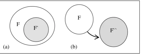
Figure 1 : Dimension reduction techniques (a) Feature Selection (b) Feature Extraction
The number of extracted features might or might not be less than the original number of features. By construct, feature selection techniques applied to select a smaller subset of useful features out of the original ones. Not only their numbers matter but also the resulting features themselves does also. For instance, interpreting the output of algorithms based on feature extraction can often prove to be problematic. The transformed features may have no physical meaning to the domain expert. On the other hand, the dimensions retained by a feature selection procedure can be directly interpreted [4].
Feature selection prioritized to be the method applied in this research. The most relevant features preferred to be selected rather than being extracted. That would probably lead to a better data acquisition later considering valuable ones only. Moreover, there is a gained benefit of reducing the number of features being processed by having the same number of features. It would enhance the data processing performance consuming more reasonable less amount of time.
2.2
Evolutionary Algorithms (EAs)
Evolutionary algorithms (EAs) estimate optimal solutions to save the time that can be consumed searching all the possible solutions of a problem, brute force search. EAs used to approximate a solution that provides an acceptable rate of accuracy and avoiding misuse of resources. They implement a mechanism that simulates biological evolution, such as reproduction, mutation, recombination, and selection. Candidate solutions those are optimizing a problem play the role of individuals in a population, and the fitness - object - function determines the quality of each solution. Then, the population evolves after the repeated application of those operators [5].
That said, any EA would have three phases. Initialization is the first where the individuals of the initial population generated randomly based on the solution declaration. Each of these individuals is a solution, and it is evaluated by a fitness value in the second phase. Fitness values used to rank the solutions in the population for selection or to calculate the average fitness value of the population. The third phase has the generation of a new population by neglecting the disturbance in the existing population of solutions [6]. A population disturbed by individuals with less fitness values. Figure 2 shows the flow of applying the three phases. A new population generated repeatedly if no stopping criteria met, this scenario keeps repeating until at least one criterion satisfied. On one hand, fitness value could be calculated by a mathematical equation for example, as it also could be found through applying other methods and it would be counted as a fitness function or - as called in many literatures - object function. It can be only designed or determined after analyzing the considered problem. On the other hand,
stopping criteria could be static or dynamic. If it is static, the algorithm is permitted to run for a fixed integer of iterations. Where applying a dynamic one would allow the algorithm to
[image:2.595.326.528.120.309.2]be repeated until a specified percent of the solutions is the best found considering some percentage. Other than that, a combination of different stopping criteria could be performed as well.
Figure 2: Evolutionary algorithms’ phases
To use an evolutionary algorithm for dimension reduction and optimization problems, the solutions representation must be determined first based on the characteristics of the specified evolutionary algorithm. The population generated by these algorithms may have infeasible solutions. Therefore, choosing a solution representation is very critical that is more probable to produce feasible solutions. The solution representation can be direct or indirect, but each of the solution population generated must be able to be decoded into a feasible solution. A decoding procedure often used along with any indirect representation in complex problems to convert it into a possible solution. Hence, the fitness function can be evaluated once that solution decoded. Considering any features describing data to be reduced, each member of an EA population is representing a subset of these features. To give an illustration of that, a population member can be formed through a random sequence of 0's and 1’s where its length equals the primary number of features. These zeroes and ones are performing as on and off switchers marking the presence of the features whether to be part of the resulting subset or not. If it is “0” then the corresponding feature is going to be neglected in that subset and it will be included if it is “1”. Moreover, two important parameters rather than the solution representation must be defined primarily. Those Parameters are the maximum number of iteration and the population size. Both have a major influence on the quality and accuracy of the solution and the time it would take to be found. These values are almost always determined empirically through pilot runs in practice even though there are many values suggested and can be tested as well.
Considering the literature [7] [8] [9], it is apparently that evolutionary algorithms are practical solution to get global optimal solutions for real world problem. Among many EAs, Particle Swarm Optimization (PSO), Differential Evolution (DE) and Genetic Algorithm (GA) are the most dominant ones. GA is the proposed model’s EA involved. In the GA strategy, solutions decoded first into binary numbers to create a population. Then each of these solution, called chromosome also, converted using specified lower and upper limits into real value if needed. After that, each chromosome is evaluated by a fitness function. The GA begins its search with a randomly generated population of designs space. This
Start EA
Generate Initial Population
Stop Criterion?
Fitness Value Evaluation
Stop EA Generate New Population
No
Yes
(a) (b)
F F`
F
13 population evolves a generation where an optimal solution
possibly would occur. It uses three operators to process its populations from one generation to another: selection, crossover and mutation. The selection operator comes first, and it selects good chromosomes in a generation and forms the crossover population. The second operator, crossover, transmits the best features of the current population to the next population, those with better fitness values. For instance, a new chromosome could be composed out of two of the best current ones by loading half of its features from some of the first one features where the other half would be filled by the other chromosome features. The formed chromosome does not guarantee a higher fitness value. The goodness of a chromosome could be a result of a certain combination of its features and this combination could be lost during this process. The crossover rate is normally quite large and is between 70% and 95% of the total population while the rest of the following population content would be kept unchanged. The last operator, mutation, supports diversity in the features of the population and using mutation probability to restrict the algorithm from getting trapped in a local minimum. These steps keep repeating until some stop criterion met.
2.3
Classification
It is a data mining task of predicting the value of a categorical variable, target or class, by building a model based on one or more numerical and/or categorical variables, predictors or attributes. Applying classification concept to different subsets of features would nominate the best to be investigated to produce the most possible accurate results. These results used to train classifiers by applying supervised machine learning algorithms. These classifiers called supervised classifiers and can be categorized in general into linear and non-linear methods. On this paper, a linear method applied using linear functions to distinguish classes, Linear Discriminant Analysis (LDA). It yields a better performance than many other classifiers. This classifier goes under covariance matrix category which is one of four distinct categories such as frequency table, similarity functions and others.
LDA is a supervised learning and a classification method originally developed in 1936 by R. A. Fisher. It is simple, mathematically robust and often produces models whose accuracy is as good as more complex methods. It is based on the concept of searching for a linear combination of variables (predictors or features) that best separates two classes (target and non-target for example). To declare the idea of being separated, Fisher defined the following score function:
𝑍 = 𝛽1+ 𝛽2𝑥2+ … + 𝛽𝑑𝑥𝑑
𝑆 𝛽 = 𝛽𝑇𝜇1− 𝛽𝑇𝜇2
𝛽𝑇𝐶𝛽 score function
𝑆 𝛽 = Ζ 1− Ζ 2
𝑉𝑎𝑟𝑖𝑎𝑛𝑐𝑒 𝑜𝑓 𝑍 𝑤𝑖𝑡𝑖𝑛 𝑔𝑟𝑜𝑢𝑝𝑠
Considering the score function, the main matter is to estimate the linear coefficients that maximize it and that can be solved by these equations:
𝛽 = 𝐶−1 𝜇
1− 𝜇2 Model coefficients
𝐶 = 𝑛 1
1+ 𝑛2 𝑛1𝐶1− 𝑛2𝐶2 Pooled covariance matrix where:
𝛽: 𝐿𝑖𝑛𝑒𝑎𝑟 𝑚𝑜𝑑𝑒𝑙 𝑐𝑜𝑒𝑓𝑓𝑖𝑐𝑖𝑒𝑛𝑡𝑠 𝐶1, 𝐶2: 𝐶𝑜𝑣𝑎𝑟𝑖𝑎𝑛𝑐𝑒 𝑚𝑎𝑡𝑟𝑖𝑐𝑒𝑠
𝜇1, 𝜇2: 𝑀𝑒𝑎𝑛 𝑣𝑒𝑐𝑡𝑜𝑟𝑠
The discrimination effectiveness can be asserted by calculating the Mahalanobis distance between two groups. If it is greater than three, then it means that in two averages differ by more than three standard deviations, and the overlap (probability of misclassification) is quite small.
Δ2= 𝛽𝑇 𝜇 1− 𝜇2
Δ: Mahalanobis distance between two groups That to end, a new point is classified by projecting it on the direction that maximally separating the classes and classifying it as c1 if:
𝛽𝑇 𝑥 − 𝜇1− 𝜇2
2 > log 𝑝(𝑐1)
𝑝(𝑐2)
Implementing LDA as a fitness - object - function of an EA requires more further steps. Each proposed solution would be examined through LDA to get the classifier trained then later tested. While testing, classification errors are calculated then divided by the size of test data. The result is forming a classification accuracy returned to the EA to be assigned as a fitness value to that solution.
2.4
High-Performance Computing (HPC)
High-performance computing (HPC) is the use of parallelism for running advanced application programs efficiently, reliably and quickly. The term applies especially to systems that function above a teraflop or 1012 floating-point operations per second. The term HPC is occasionally used as a synonym for supercomputing, although technically a supercomputer is a system that performs at or near the currently highest operational rate for computers. Some supercomputers work at more than a petaflop or 1015 floating-point operations per second.14
3.
METHODOLOGY
3.1
Resources and Programming Models
3.1.1
Machine and HPC models and languages
This research runs its code on Fujitsu PRIMERGY CX400, Intel Xeon E5-2695v2 12C 2.4GHz, Intel True Scale QDR. This machine called Aziz, launched on June 01, 2015 at King Abdul-Aziz University [12] and considered to be one of the top 500 supercomputers [13]. Message Passing Interface (MPI) model implemented and the system implemented in C and C++ programming languages.3.1.2
Library used
Boost from boost.org used within the implementation of this paper proposed model coding. It is a free peer-reviewed portable C++ library. It provides support for tasks and structures such as linear algebra, pseudorandom number generation, regular expressions, image processing, multithreading, and unit testing. It contains over eighty individual libraries. Most of the Boost libraries allowed to be used with both free and proprietary. In the LDA classifier Boost is there. It has been used to implement matrices basically as the library covers the common basic linear algebra operations on vectors and matrices: reductions, addition, subtraction, multiplication with a scalar, inner and outer products of vectors. The connection between containers, views and expression templated operations is a regularly STL conforming iterator interface. via operator overloading and efficient code generation. Therefore, it plays a major rule being employed in the models' design and execution.
3.2
Proposed model
In this model, a parallel version of GA implemented using a migration technique called islands. An island represents one of the nodes, single computing resource, performing the algorithm in parallel. The GA population is distributed and divided equally where each node would have its own subpopulation. The more nodes involved in the process the bigger population is there. For an instance, 4 nodes would work on a population of 4 into 50 members where 64 nodes will have 64 into 50 members to work with and the same goes for any number of nodes. After each generation, some members would migrate from one island to its neighbors in a ring arrangement. The least fit member of the current subpopulation migrates in a clockwise to be the least fit one of the neighbor to the right, where the fittest member migrates in a counterclockwise to be the fittest one of the left neighbor. This concept enables the nodes to communicate, thus, they wouldn't replicate each other which would save the overall time consumed. An important note to mention that GA is assigning the member with the highest fitness value as the fittest one where the one has the lowest value to be the least.
3.3
Dataset Involved
A standard dataset used while developing the proposed model that is the CorrAL [14] [15]. CorrAL dataset considers an artificial domain and consists of 128 samples each of A0, A1, B0, B1, Irr, R, C. The target concept is (A0^A1) V (B0^B1), Irr is irrelevant, and R is an attribute highly correlated with the label C but with 25% error rate. This solution generated by GA comprised of zeroes and ones where 0's represent that the features going to be ignored where the 1's reflects the considered ones. Getting the dataset that has the considered features only is the next stage. Then, resulted dataset goes through the classification process that would define different samples for the specified classier training and testing.
3.4
Test Scenario
The CorrAL dataset tested on the feature selection model based on HPC techniques. The stopping criterion used in the EAs, in general, was the number of iterations or generations processed. Three values set to this parameter: 1, 2 and 4 iteration/s. For the set of processors varying numbers have been tested. The one to start with was 4 processors to check the effect of using such small number so that the effect of running larger numbers of processors. Other numbers of processors planned to be involved are 128 processors as a large one and 64 to represent a middle point between both of the previous numbers.
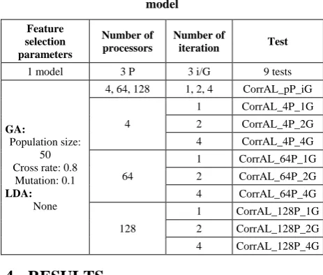
In sight of the mentioned parameters, there was nine tests, Table 1. There is one proposed model running on a single dataset utilizing three values of the GA stopping criterion and three sets of processors.
Table 1: CorrAL dataset tests on the feature selection model
Feature selection parameters
Number of processors
Number of
iteration Test
1 model 3 P 3 i/G 9 tests
GA:
Population size: 50 Cross rate: 0.8
Mutation: 0.1
LDA:
None
4, 64, 128 1, 2, 4 CorrAL_pP_iG
4
1 CorrAL_4P_1G
2 CorrAL_4P_2G
4 CorrAL_4P_4G
64
1 CorrAL_64P_1G
2 CorrAL_64P_2G
4 CorrAL_64P_4G
128
1 CorrAL_128P_1G
2 CorrAL_128P_2G
4 CorrAL_128P_4G
4.
RESULTS
[image:4.595.312.544.266.463.2]In this section, the results of testing the feature selection model over the CorrAL standard dataset shown. Then, their performances explored. The following table and charts summarize those of test scenarios described earlier. Table 2 displays the time results of applying the model to the CorrAL dataset and the improvement rates. These improvement rates calculated based on the results related to the processing time of performing a sequential version of the model on normal computing facilities. That would be 6 to 60 times the time spent by the parallel version of the same model proposed here.
Table 2: Model's time results on CorrAL P Accuracy No of features Time Time Imp.
4 85.56 4.33 0.97 98.02
64 86.67 3.33 4.88 90.04
128 86.67 4.00 9.76 80.09
15 dataset has only 128 samples. Thus, 4 processors as an
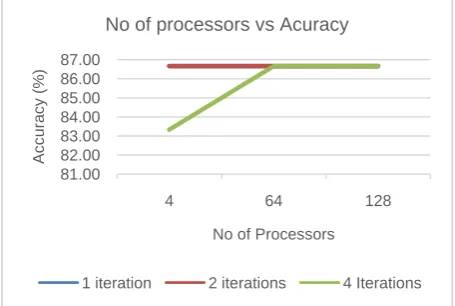
[image:5.595.315.543.101.256.2]instance (a small set of processors) achieved the best results. Even though, the model performs its best in the case of 4 processors taking less than 2% of the original time spent earlier before applying this model. The following Figure, Figure 3, the detailed results of accuracy for the tests showing the slight variation. It shows that higher number of iterations involving a small number of processors might lead to lower accuracy rate. Besides, using a moderate number of iterations and processors would likely to produce similar rates of accuracy.
Figure 3: The feature selection model accuracy results involving different numbers of processors (4, 64, 128) on
CorrAL distinguishing the results for each number of iterations (1, 2, 4)
In
[image:5.595.53.281.199.352.2]Figure 4, it indicated clearly that executing higher number of iterations lead to more processing time. The same goes for employing more processors for the same number of iterations. Thus, different numbers of iterations and processors should be tested over the data to determine the most suitable set. It is required to satisfy the tradeoff between timing and computational costs achieving an acceptable rate of accuracy.
Figure 4: The feature selection model time results involving different numbers of processors (4, 64, 128) on
CorrAL distinguishing the results for each number of iterations (1, 2, 4)
The last Figure, Figure 5, illustrates the final results achieved by the feature selection model proposed in this paper. It shows the considerable reduction in the processing time. The model
attempts to find the least possible number of features maintaining an acceptable rate of accuracy.
Figure 5: The average time results of applying feature selection model based on number of processors (1, 4, 64,
128) on CorrAL
5.
CONCLUSION
In this paper, a model proposed to solve the curse of dimensionality problem based on feature selection methods and HPC techniques. GA as a search algorithm and LDA as a classifier formed the feature selection method and MPI were the technique applied to perform the parallelism concept of HPC. Both notions formed the model then it has been implemented in C/C++ programming languages. Later, the model tested on a standard dataset called CorrAL. As a result, it saves in average 89% of the time used to be consumed while using conventional computing capabilities. It also eliminates more than the third of the features maintaining an accuracy rate of 86% on average.
The model can run larger sizes of data and be applied on higher numbers of processors. It is expected to accomplish similar or even better results as the ones attained in this paper running over considerably large sets of data.
Several feature selection models can be formed following the same strategy employed. Different classifiers of the same category selected, linear, other categories, or uncategorized classifiers as well. On the other side, other search algorithms could be involved instead of the one employed in the discussed model earlier. EAs rather than GA could be concerned to be implemented and tested for further analyses.
6.
ACKNOWLEDGMENTS
All computations were performed on Aziz Supercomputer at King Abdul-Aziz university's High- Performance Computing Center (HPCC), http://hpc.kau.edu.sa . The authors would like to acknowledge the computer time and technical support provided by the center.
7.
REFERENCES
[1] Fodor, Isola K. "A survey of dimension reduction techniques." (2002).
[2] Cunningham, Pádraig. "Dimension reduction. "Machine learning techniques for multimedia. Springer Berlin Heidelberg, (2008). 91-112.
[3] Kamel, Mahmoud I., and Anas A. Hadi. Improving P300 Based Speller by Feature Selection. Journal of Medical Imaging and Health Informatics 4.4: 469-487, 2014. 81.00
82.00 83.00 84.00 85.00 86.00 87.00
4 64 128
Ac
c
uracy
(%
)
No of Processors No of processors vs Acuracy
1 iteration 2 iterations 4 Iterations
0.00 5.00 10.00 15.00 20.00
4 64 128
Tim
e
(m)
No of processors No of processors vs Time
1 Iteration 2 iterations 4 iterations
0 10 20 30 40 50 60 70
1 4 64 128
Tim
e
(s)
[image:5.595.52.281.515.683.2]16 [4] Cunningham, Pádraig. Dimension reduction. Machine
learning techniques for multimedia. Springer Berlin Heidelberg, (2008).91-112.
[5] Yu, Xinjie, and Mitsuo Gen. Introduction to evolutionary algorithms. Springer Science & Business Media, (2010).
[6] Xin-She Yang, Engineering Optimization – An
Introduction to Metaheuristic Applications. John Wiley & Sons, Hoboken, New Jersy, (2010).
[7] K Y Lee, M.A. El-Sharkawi, “Modern Heuristic Optimization Techniques” IEEE press and Wiley – InterScience, New Jersy, (2008).
[8] Rody P S Oldenhuis, “Trajectory Optimization of a mission to the Solar Bow shock and minor planets”, MSc thesis report, Delft University of Technology, Netherlands, (Jan 2010).
[9] Kachitvichyanukul, Voratas. Comparison of Three Evolutionary Algorithms. Industrial Engineering & Management Systems 11.3 (2012). 215-223.
[10] Umbarkar, A. J., M. S. Joshi, and P. D. Sheth. OpenMP Dual Population Genetic Algorithm for Solving Constrained Optimization Problems. International
Journal of Information Engineering and Electronic Business (IJIEEB) 7.1: 59, (2015).
[11] Slate's article Stephen: Wolfram's New Programming Language: He Can Make The World Computable, March 6, 2014. Retrieved on 14-05-2015.
[12] Fujitsu Supports King Abdul-Aziz University Research Capabilities with New Supercomputing System. Press release. King Abdul-Aziz University, Fujitsu Limited. Jeddah and Tokyo, June 01, 2015
[13] Top 500, The List. http://www.top500.org/site/50585 , (2015).
[14] John, Kohavi, and Pfleger, Irrelevant features and the subset selection problem. Machine Learning: Proceedings of the Eleventh International Conference, available at http://robotics.stanford.edu/~ronnyk. Last access: 10/22/2017.
[15] Datasets from UCI. SGI, Silicon Graphics International Corp. https://www.sgi.com/tech/mlc/db/ . Last access: 10/22/2017.