Argument Generation for a Biomedical Domain

(1)

ABSTRACT

NAVORAPHAN, KANYAMAS. Argument Generation for a Biomedical Domain. (Under the direction of Nancy L. Green and James C. Lester.)

Discourse generation is a critical task of natural language generation. In this thesis, we

introduce an approach to discourse generation for qualitative causal probabilistic domains

that incorporates argumentation into the generation process. The discourse generation

process uses three modules: a qualitative causal probabilistic domain model, a genre-specific

discourse grammar, and a normative argument generator. The model of discourse generation

has been implemented for the domain of clinical genetics. In conjunction with GenIE, a

prototype intelligent system for generating the first draft of a patient letter on behalf of a

genetic counselor, the discourse grammar exploits general information about clinical genetics

as well as documentation about a specific patient's case provided by a genetic counselor, to

create discourse plans. The argument generator generates arguments for the claims passed to

it from the discourse grammar using domain-independent argument strategies. An important

contribution of the thesis is a modification of the argument generator to support interactive

(2)

Argument Generation for a Biomedical Domain

by

Kanyamas Navoraphan

A thesis submitted to the Graduate Faculty of North Carolina State University

In partial fulfillment of the Requirements for the degree of

Master of Science

Computer Science

Raleigh, North Carolina

2008

APPROVED BY:

___________________________ ___________________________

Dr. Robert D. Rodman Dr. R. Michael Young

___________________________ ___________________________

(3)

DEDICATION

To life, and what remains of it

Carpe diem: Seize the day

(4)

-BIOGRAPHY

Kanyamas Navoraphan was born in Bangkok, Thailand, in 1976. She received her Bachelor

of Arts degree in English from Chulalongkorn University, Bangkok, Thailand in 1996. She

then obtained a second Bachelor of Science degree in Computer Science from University of

Hawaii at Manoa in Honolulu, Hawaii in 2000. After working as a Software Engineer with

Synopsys Inc., Mountain View, California for five years, from July 2000 to August 2005, she

joined the graduate program at the Computer Science Department in North Carolina State

University in the fall of 2005. Her dream is to combine the knowledge in both the language

and the computer science fields in the area of natural language processing, specifically

(5)

ACKNOWLEDGEMENTS

I would like to express my sincere gratitude to the following people without whose help and

support I could not have achieved what I have.

My advisor, Dr. Nancy L. Green, for her continued guidance and support, and especially for

spending endless hours perfecting my thesis.

My co-advisor, Dr. James C. Lester, for introducing me to Dr. Green, and for his help in

reviewing the final draft of my thesis.

The members of my committee, Dr. Robert D. Rodman and Dr. R. Michael Young for their

academic support.

My project partner, Rachael Dwight, for insightful discussions throughout the course of the

project.

My friend, Valuncha Paterson, for her help in formatting my thesis, and for giving me the

much-needed encouragement throughout the course of my thesis writing.

My friend, Jeremy Paterson, for his help in reviewing my thesis.

My friend, Emilie Wang, for her help in providing me valuable feedbacks during my thesis

defense preparation.

My parents, for providing me the greatest gift of education, for their unconditional love and

understanding, and for being there for me, always.

The rest of my family and friends, for their love and support, without whom I would not be

who I am today.

This material is based upon work supported by the National Science Foundation under

(6)

LIST OF TABLES

Table 2-1: A full set of node types and their descriptions [Green, 2005]. ...9

Table 2-2: Domain definition and corresponding scalar values. ... 10

Table 4-1: List of nucleus-satellite RST relations used in the Discourse Grammar. ... 33

Table 4-2: List of multinuclear RST relations used in the Discourse Grammar. ... 34

Table 5-1: The six elements of argument in Toulmin’s argument structure [Toulmin, 2003]. ... 39

Table 6-1: List of possible choices and corresponding actions in Argument Generation state. ... 60

Table A-1: Non generic events in the Cystic Fibrosis KB. ... 97

Table A-2: Generic events in the Cystic Fibrosis KB. ... 99

Table A-3: Non-generic events in the Achondroplasia KB. ... 100

Table A-4: Generic events in the Achondroplasia KB. ... 102

Table A-5: Non-generic events in the Familial Hypercholesterolemia KB. ... 103

Table A-6: Generic events in the Familial Hypercholesterolemia KB. ... 105

Table A-7: Non-generic events in the Phenylketonuria KB.... 105

(9)

LIST OF FIGURES

Figure 2-1: Examples of S+andS– relations. ... 14

Figure 2-2: Example of a Y+relation. ... 15

Figure 2-3: Example of a Y–relation. ... 16

Figure 3-1: The pretest state of the Cystic Fibrosis KB. ... 19

Figure 3-2: The posttest state of the Cystic Fibrosis KB. ... 20

Figure 3-3: The future state of the Cystic Fibrosis KB. ... 21

Figure 3-4: The pretest state of the Achondroplasia KB. ... 23

Figure 3-5: The posttest state of the Achondroplasia KB. ... 24

Figure 3-6: The future state of the Achondroplasia KB. ... 25

Figure 3-7: The pretest state of the Familial Hypercholesterolemia KB. ... 26

Figure 3-8: The posttest state of the Familial Hypercholesterolemia KB. ... 27

Figure 3-9: The posttest state of the Phenylketonuria (PKU) KB. ... 28

Figure 3-10: The future state of the Phenylketonuria (PKU) KB. ... 29

Figure 4-1: The discourse generation process. ... 31

Figure 4-2: A rough organization of the dplan. ... 35

Figure 5-1: The RST representation of an argument [Green, 2007]. ... 40

Figure 5-2: The applicability constraint of the E2C argument scheme. ... 41

Figure 5-3: Constraints of a variant of the E2C argument scheme. ... 42

Figure 5-4: Another variant of the E2C argument scheme. ... 43

Figure 5-5: The three applicability constraints of the NE2C argument scheme. ... 44

(10)

Figure 5-7: The E2XORC argument scheme. ... 47

Figure 5-8: A sample scenario illustrating a variant of the ELIM argument scheme. ... 48

Figure 5-9: An example of a complex argument generation. ... 50

Figure 5-10: The data exchange between the discourse generator and the argument generator.... 51

Figure 5-11: An RST tree before and after pruning. ... 56

Figure 6-1:FSM representing the interactive argument generator’s architecture. ... 58

Figure 6-2: Detailed FSM during the Argument Generation state.... 61

Figure 6-3: Example user interaction during KB, KB state, and node selections. ... 62

Figure 6-4: Argument Listing Format. ... 63

Figure 6-5: An example of user interaction during warrant selection. ... 63

Figure 6-6: Sample Test KB. ... 68

Figure A-1: Section 1 of the Cystic Fibrosis dplan. ... 87

Figure A-5: Section 1 of the Achondroplasia dplan. ... 91

Figure A-8: Section 1 of the Familial Hypercholesterolemia dplan. ... 94

Figure A-9: Section 2 of the Familial Hypercholesterolemia dplan. ... 95

(11)

(12)

CHAPTER 1 INTRODUCTION

The goal of this research is to develop GenIE, a prototype intelligent system for generating

the first draft of a patient letter on behalf of a genetic counselor, using general information on

clinical genetics as well as specific documentation about the patient‟s case provided by the

genetic counselor. The work done for this thesis focuses on the reimplementation of the

GenIE prototype first described in [Green, 2006], using a new discourse grammar that

generates discourse plans employing Rhetorical Structure Theory (RST) relations [Mann and

Thompson, 1988] as specified in [Green, 2007]. The work also includes an implementation

of domain models for four new genetic diseases partly based on case studies in [Korf, 2000]

and [Nussbaum, McInnes, and Willard, 2001], and implementation of an interactive

argumentation driver.

Like many other natural language generation (NLG) systems [Reiter and Dale, 2000], GenIE

uses a nonlinguistic domain model. Generation is performed in two stages: discourse generation, and then linguistic realization. The scope of this thesis covers the domain model

(13)

The domain model is a causal probabilistic knowledge base, designed specifically to store information related to clinical genetics. Discourse generation is divided into two separate parts, namely the discourse grammar, and argument generation. The output from discourse generation is in the format to be used as input to the linguistic realizer at a later time.

Because the work on linguistic realization is incomplete at this point, as part of the work done on this thesis, we have also implemented an interactive driver for the argument

generator that can be used to partially validate the intermediate outputs as far as argument

generation is concerned. The last part of this thesis describes the interactive driver. All

implementation for this thesis was done using the logic programming language Prolog.

1.1. Genetics Background

According to [Baker et al., 2002; Harper, 1998], genetic counseling is the process by which a patient who is at risk of a genetic disorder seeks advice on how to deal with such disease

from a genetic counselor. The advice ranges in nature from the general characteristics of the

disease, its symptoms and consequences, the probability of developing and transmitting it, as

well as the options and procedures available to prevent or treat the disease. Genetic

counselors generally work as members of a healthcare team to identify families at risk and

investigate problems present in the family. Then, they go on to meet with the patient and his

family to review available testing options, discuss risk of complications, interpret test results,

(14)

An important task performed by a genetic counselor is to educate the patient about his

disease. It is thus important that the counselor be able to communicate in terms that are

comprehensible to a lay audience. Sending letters with details summarizing the services and

information provided is a way to keep the patient informed about his health conditions.

Adequate understanding of the health conditions in turn enables the patient to be more

actively involved in his own healthcare. This type of standard document designed to record

the counselor‟s reasoning for medical as well as legal purposes is called a patient letter.

1.2. Related Work

Argument generation is among the topics that attract research interest in the area of NLG due

to the fact that argument is, by nature, a highly structured form of text [Reed and Long, 1998]. Zukerman et al. have done work on an argument generation system called NAG (Nice Argument Generator) [Zukerman et al., 2000], which relies on domain models that are based on a Bayesian Network formalism. Unlike NAG, GenIE‟s domain model uses a qualitative

probabilistic network formalism as its main representation. Also, whereas NAG generates

arguments using standard deductive and Bayesian argumentation strategies, GenIE‟s

argument strategies are based on analysis of a corpus of genetic counseling patient letters.

[Reed and Long, 1997] present a framework that supports the modeling of argument structure

using a hierarchical planner. First, an abstract plan is generated through operators that encode

deductive argument schemes. These operators complete the plan by fulfilling its

(15)

maximize persuasive effects as well as coherency of the argument. In their subsequent work,

[Reed and Long, 1998] describe Rhetorica, an abstraction-based planning system that uses deductive, refutation, and inductive generalization operators to generate complex argument

structure. The planning occurs at a level that is more abstract than RST. This extra layer is

introduced specifically to represent argumentative relationships that cannot be expressed with

RST. Like Rhetorica, GenIE also uses argument schemes to support its generation of arguments at a level that is more abstract than RST.

[Branting et al., 1999] describe a legal document drafting system that relies on both domain knowledge as well as discourse knowledge to generate legal arguments. Similar to GenIE,

the system uses a discourse grammar to define the organization of the document, and then

fills in the content with legal reasoning. However, in GenIE, we separate the task of domain

reasoning from argument generation.

[Grasso et al., 2000] present Daphne, a nutrition counseling system that uses an argumentation theory framework to provide healthy nutrition advice. Like GenIE, though the

system has been implemented to work in a healthcare-related domain, the domain knowledge

was kept as a well-defined component separate from the argumentative tactics that are

expressed in general terms and thus make Daphne extendable to other domains. Unlike

GenIE, Daphne is intended to generate persuasive arguments in interactive dialogue with

users based on informal argumentation theories [Perelman and Olbrechts-Tyteca, 1969]

(16)

The goal of the GenIE project [Green, 2005; Green, 2006; Green, 2007; Green, submitted] is

to investigate generation of scientific arguments for lay audiences. The testbed for the

research is the development of a natural language generation system for drafting genetic

counseling patient letters. After collecting a corpus of patient letters from genetic counselors,

Green developed and formally validated the inter-coder reliability of a coding scheme for

annotating genetic counseling patient letters [Green, 2005]. The coding scheme provides a

conceptual model of single-factor genetic disease that is used in expert-lay communication in

this domain. This conceptual model of genetic disease was used to guide design of the

domain model in the GenIE architecture [Green, 2006]. The domain model is represented as

a qualitative probabilistic network. This architecture also makes use of a genre-dependent

discourse grammar and non-genre-specific argument schemes that map formal

(domain-independent) properties of a qualitative probabilistic network to functional elements of

Toulmin‟s [Toulmin, 2003] model of argument (e.g., data, claim, and warrant). In a study of

pragmatic features of argumentation in the corpus, [Green, 2007] presents extensions to

Rhetorical Structure Theory [Mann and Thompson, 1988] incorporating Toulmin‟s

components of arguments. Finally, [Green, submitted] presents a dialogue game for

challenging and asking follow-up questions to arguments generated in the GenIE

(17)

1.3. Thesis Organization

This thesis is organized as follows: Chapter 2 discusses the domain model. Chapter 3

describes in detail the four knowledge bases used to test the system. Discourse generation is

presented in two chapters: Chapter 4 presents the first part of generation using the discourse

grammar, and Chapter 5 presents the second part, argument generation. Chapter 6 describes

the interactive driver, a tool used to test the functionality of the system as far as argument

generation is concerned. Chapter 7 concludes the discussion and notes directions for future

(18)

CHAPTER 2 DOMAIN MODEL

The domain model is a knowledge base (KB) containing information about a patient‟s case

and general information about genetic disease. This chapter describes the implementation of

the KB as a qualitative probabilistic network (QPN). The next chapter explains the four KBs

implemented for this thesis.

2.1. Qualitative Probabilistic Network

A qualitative probabilistic network is a directed acyclic graph whose nodes represent random

variables and whose edges represent the dependencies between the random variables. The

idea of a QPN was introduced as an abstraction of a Bayesian Belief Network, where

numerical probability relations are replaced with qualitative influences and synergies

[Wellman, 1990, Druzdzel and Henrion, 1993]. QPNs are thus ideal for situations where

numerical probabilities are either unavailable or unnecessary to complete the tasks at hand.

For GenIE, we need a model of the patient‟s case that can be used to generate arguments in

the patient letters for the diagnosis and other conclusions of medical experts. For example,

given the diagnosis reported by the genetic counselor, GenIE will search its KB for evidence

(19)

domain reasoning, it is sufficient for the domain model in GenIE to use qualitative

constraints as described in [Green, 2006]. The constraints are described in section 2.3.

2.2. Implementation

A KB contains one or more QPNs. Each network is a directed acyclic graph (DAG). Each

graph describes the disease at a specific period of time. Each node of the DAG represents

either a random or a decision variable, depending on its type. In GenIE, a random variable

node is simply called a node whereas a decision variable node is called a dnode. Each node consists of five different attributes, namely

node identifier (ID)

type

domain

role

node description

Node IDs are unique within each KB. For consistency purposes, we use the same naming

convention across all KBs. The first part of a node ID represents its type, whereas the second

part denotes the genealogical role of the person the node is describing, followed by an

optional third part which is a numerical index to distinguish a group of nodes that refer to the

same abstract variable type for the same family member. For example, we can expect a node

(20)

genotype). Similarly, the nodes sp1 and sp2 will most likely describe two different symptoms (s for symptom) the proband is experiencing.

Table 2-1: A full set of node types and their descriptions [Green, 2005].

Type Description node dnode

history Demographic or predispositional factor (e.g., gender,

ethnicity, age, family history of a specific mutation,

environmental risk factor)

yes no

genotype A pair of alleles1 of a gene inherited from parents yes no genotype_germline A pair of alleles of a gene resulting from mutation rather

than inheritance

yes no

event Event that results in a change in an individual‟s genotype at

different points in his life cycle and/or in different cells

yes no

biochemistry Manifestation of an individual‟s genotype at the biochemical

level, e.g., a shortened protein

yes no

physiology Manifestation of an individual‟s genotype at the

physiological level, e.g. in metabolism

yes no

symptom Manifestation of an individual‟s genotype that is observable

without performing a test, e.g., some type of birth defects

yes no

test Event of performing a test no yes

test result Result of a test yes no

complication Undesirable side effect of a test, e.g., fetal damage yes no

1

(21)

Table 2-1 (continued).

Type Description node dnode

behavior An activity performed by an individual which can be

observed

yes no

treatment A specific procedure used for the cure of a disease or a

condition

no yes

A small set of node types was identified in [Green, 2005] to cover the extent of KB contents

used in this research. Table 2-1 lists the full set of all node types including their brief

descriptions. The set reflects a simplified model used by genetic counselors to communicate

with their clients.

The domain attribute of a node indicates the range of values the node is allowed to take.

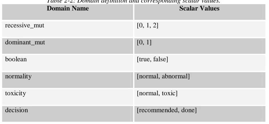
Table 2-2 below shows the domain definition with corresponding scalar values.

Table 2-2: Domain definition and corresponding scalar values.

Domain Name Scalar Values

recessive_mut [0, 1, 2]

dominant_mut [0, 1]

boolean [true, false]

normality [normal, abnormal]

toxicity [normal, toxic]

(22)

Table 2-2 (continued).

Domain Name Scalar Values

nninteger any non-negative integer

real_0_1 any real number between 0 and 1

The role and node description attributes of a node indicate the role in the family tree and the specific concept represented by the node, respectively. Every KB consists of one or more

node definitions for the role proband. Following standard convention in genetics, other roles such as father, mother, future_sibling, and offspring are specified relative to the proband. Like a node‟s ID, its role and description together can be used to uniquely distinguish one

node from the others.

A graph is defined by the KB state at a particular time (pretest, posttest, future, etc.), and a

list of arcs it contains. Each directed arc that connects one node to another has a unique

identifier with respect to the KB. The same arc may occur in more than one graph, and does

not necessarily occur in every graph. Each graph has one root node called superroot, of which other nodes are descendants. This special dummy node was introduced in the effort to

keep each graph a connected network2. Without superroot, we would have ended up with dangling decision nodes, specifically dnodes of type test, which typically do not connect to any other nodes in the pretest graphs. This will be illustrated in the next chapter.

2

(23)

A node may have different states, representing its possible states at a specific time. Each

node state is explicitly defined with three components, including a node ID, a KB state, and

an assignment list. In the current implementation, the assignment list contains at most one

element. Each element of an assignment list is a tuple, consisting of an assignment and its

corresponding probability. An assignment is in the form of [Op, Value] for numeric values, where Op is one of {=, >=, =<, >, <}, or Value alone if nonnumeric. A probability is of the form [Ptype, Pvalue] where Ptype is the name of a defined probability value format, and

Pvalue is the probability value. The probability value represents the degree of belief in different states of a node. Probability type can be either qualitative or quantitative. In the

current implementation, Ptype is qualitative, with an allowable scale of [very_low, low, high,

very_high]. For decision nodes where no probability is required, an empty list is put in the place of its probability. Examples of state definitions include the following:

state(tstp, pretest, [[recommended, []]]).

Paraphrase: In the pretest graph, the proband’s test is recommended. state(sm, posttest, [[false, [qual, high]]]).

Paraphrase: In the posttest graph, the belief that the mother does not have symptoms is high.

state(gp, future, [[[=, 2], [qual, very_high]]]).

(24)

In the current implementation, no more than one state predicate is defined per variable per KB state. However, it is possible for a variable‟s state to change from one KB state to the

next. For example, in the pretest KB state, the state of a test node is generally defined to be

recommended, whereas in the posttest state, the node‟s state usually changes to done.

Apart from concepts represented by nodes and the relationships among them represented by

arcs, the domain model also stores epidemiological statistics related to the concepts used in

the network. For example, in the Achondroplasia KB (described in the next chapter), we

have:

statistic(cprob([[G, [=, 1]]], [range, [0.03, 0.07]], [[C, true]]), research) :- node(G, genotype, dominant_mut, Who, ‘FGFR3’),

node(C, complication, Boolean, Who, ‘sudden death in first year’). P(sudden death in first year = true │FGFR3 genotype = 1) = 3-7 %

Paraphrase: The rate of sudden death during the first year for Achondroplasia patient having 1 mutation of the FGFR3 genotype is 3-7 %.

The information, though it plays no role in domain reasoning, will be used as backing for an

argument. This process will be described in detail in the next chapter.

For information that is neither a fact nor derivable by argument, the domain model also

contains a status predicate to indicate that it is assumed. For example, in the Cystic Fibrosis KB (described in the next chapter), we have:

(25)

2.3. Qualitative Relations

To support reasoning, the domain model uses qualitative constraints based upon formal

relations of qualitative influence, product synergy, and additive synergy [Druzdzel and

Henrion, 1993]. In this section, we describe the constraints used in the four KBs covered in

this thesis.

Figure 2-1: Examples of S+andS– relations.

Nodes are connected to one another by directed arcs that represent a qualitative influence,

either positive or negative. A qualitative influence from node A to node B expresses how the value of A influences the probability of a value of B. Specifically, node A having a positive qualitative influence on node B, denoted S+ ([A, VA], [B, VB]), means that the state of A

reaching its threshold value VA makes it more likely for Bto reach its threshold value VB. For

example, a parent having one or more mutated alleles of the CFTR gene increases the

likelihood that the offspring will inherit one mutated allele from that parent. On the other gp

proband: CFTR

S+

S+([gm, [≥, 1]], [gp, [≥, 1]])

trtp

proband: lung‟s transplantation

cp

proband: respiratory failure

S–

S– ([trtp, done], [cp, true]) gm

(26)

hand, node C having a negative qualitative influence on node D, denoted S– ([C, VC], [D, VD]), means that the state of C reaching its threshold value VC makes it less likely for D to

reach its threshold value VD. For example, a lung transplantation done on a patient makes it

less likely he will experience a respiratory failure.

Figure 2-2: Example of a Y+relation.

Product and additive synergies model interaction between various influences, describing the

relation between a set of variables and their direct descendant in a graph. An additive synergy

expresses how the value of nodes A and B jointly influences the probabilities of node C

[Wellman, 1990]. A positive additive synergy of nodes A and B on their common child node

C, denoted Y+ ([[A, VA], [B, VB]], [C, VC]), expresses that the state of A reaching its

threshold value VA makes it more likely for the state of B reaching its threshold value VB to

influence Cto reach its threshold value VC. For example, a CF patient having bacteria in his

lung secretion increases the chance of his viscous lung secretion resulting in a respiratory

infection. Similarly, a negative additive synergy of nodes A and B on their common child sp

proband: respiratory infection

Y+([[ep, true], [pp, true]], [sp, true])

ep

proband: bacteria in lung secretion

pp

proband: viscous lung secretion

(27)

node C, denoted Y– ([[A, VA], [B, VB]], [C, VC]), expresses that the state of A reaching its

threshold value VA makes it less likely for the state of B reaching its threshold value VB to

influence C to reach its threshold value VC. For example, a CF patient taking caloric

supplements decreases the chance of his malabsorption resulting in a growth failure.

Figure 2-3: Example of a Y–relation.

A negative product synergy of nodes A and B on their common child node C, denoted X– ([[A, VA], [B, VB]], [C, VC]), expresses that either the state of A reaching its threshold value VA or the state of B reaching its threshold value VB makes it more likely for C to reach its

threshold value VC. Negative product synergy can be used to represent mutually exclusive

alternative diagnoses that could account for the same symptom, or to represent autosomal

dominant inheritance, an inheritance pattern where inheriting one mutated allele of a

genotype (from either parent) may lead to health problems. Examples of an X– relationship

can be seen in either the Achondroplasia KB or the Familial Hypercholesterolemia KB. sp

proband: growth failure

Y– ([[trtp, done], [pp, true]], [sp, true]) pp

proband: malabsorption

trtp

proband: caloric supplements

(28)

In contrast, autosomal recessive inheritance, an inheritance pattern in which two mutated

copies of a gene, one inherited from each parent, can be represented by zero product synergy. A zero product synergy of nodes A and B on their common child node C, denoted X0 ([[A,

VA], [B, VB]], [C, VC]), expresses that together the state of A reaching its threshold value VA

and the state of B reaching its threshold value VB make it more likely for C to reach its

threshold value VC. Examples of an X0 relationship can be seen in either the Cystic Fibrosis

KB or the Phenylketonuria KB, both of which are described in the next chapter.

(29)

CHAPTER 3 OVERVIEW OF KNOWLEDGE BASES

We use a total of four sample knowledge bases (KB) to test the functionality of our system.

All KBs were partly based on case studies found in clinical genetics textbooks. Each

describes a specific patient case of a particular genetically transmitted disease which is either

autosomal recessive or autosomal dominant. In an autosomal recessive disorder, the patient

inherits the recessive trait from both parents who are carriers, each contributing one of the

similar alleles. On the other hand, in autosomal dominant inheritance, the patient needs only

one copy of the abnormal gene from either parent in order for the trait to become apparent. In

this chapter, we describe each KB in detail, and provide graphs of each KB that show the

relationships among concepts. In each graph, the blue arrows represent S+ relations, the red

arrows S–, while the X and Y relations are explicitly tagged.

3.1. Cystic Fibrosis

The Cystic Fibrosis (CF) KB [Nussbaum, McInnes, and Willard, 2001] describes a proband

who, prior to testing, was suspected of having cystic fibrosis, an autosomal recessive disorder

caused by inheriting two mutated alleles of the CFTR (cystic fibrosis transmembrane

conductance regulator) gene, one from each parent. CF is most commonly found in

Caucasian populations. The disease frequency is 1 per 2500, whereas a carrier frequency is

(30)

affected child, the risk of cystic fibrosis recurrence in future offspring is 25% [Korf, 2000].

Studies show that the false-negative rate of carrier screening is about 1-2% [Nussbaum,

McInnes, and Willard, 2001].

hm = true (high)

'N European ancestry'

gm = 1 (high)

‘CFTR’

sm = false (high)

'CF symptoms'

hf = true (high)

gf = 1 (high)

‘CFTR’

sf = false (high)

'CF symptoms'

gp = 2 (high)

‘CFTR’

bp = abnormal (high)

'CFTR protein'

pp2 = abnormal (very_high)

'pancreas enzyme level'

pp1 = true (very_high)

'viscous lung secretion'

pp3 = true (high)

'malabsorption'

sp2 = true (high)

'growth failure'

sp1 = true (very_high)

'respiratory infections'

ep1 = true (high)

'bacteria in lung secretion' a1 a2 a5 a3 a4 a6 a7 a19 a10 a20 a21 a11 a12 tstp = recommended 'sweat'

joint_resp([gm, gf], gp)

enables([ep1, pp1], sp1)

Figure 3-1: The pretest state of the Cystic Fibrosis KB.

Both parents were of northern European ancestry, but neither showed any CF symptoms. The

(31)

observed: respiratory infections and growth failure. Bacteria in the proband‟s lung secretion

is assumed to have enabled a viscous lung secretion to cause the respiratory infections. The

growth failure, on the other hand, was believed to have been caused by malabsorption

resulting from an abnormal level of pancreas enzyme due to the CFTR mutation. The clinic

recommended that a sweat test be done on the proband. Figure 3-1 illustrates the

relationships among all concepts described at this state.

hm = true (high)

gm = 1 (very_high)

‘CFTR’

sm = false (high)

'CF symptoms'

hf = 1 (high)

gf = 1 (very_high)

‘CFTR’

sf = false (high)

'CF symptoms'

gp = 2 (very_high)

‘CFTR’

bp = abnormal (very_high)

'CFTR protein'

pp3 = true (high)

'malabsorption'

sp2 = true (high)

'growth failure'

ep1 = true (high)

'bacteria in lung secretion' a1 a2 a5 a3 a4 a6 a7 a19 a10 a19 a20 a21 a11 a12

tresp = abnormal (very_high) 'NaCl level' a9 a14 a13 trtp3 = recommended 'clearance of secretions' trtp1 = recommended 'antibiotic'

tstp = done

'sweat'

enables([ep1, pp1], sp1) enables([tstp, bp], tresp)

a8

(32)

After testing, the initial diagnosis was further confirmed by the abnormal Sodium Chloride

(NaCl) level revealed by the sweat test. Two separate treatments were recommended,

including an antibiotic to help inhibit the growth of the bacteria in lung secretion, as well as a

clearance of the secretions. Figure 3-2 shows the KB at this particular state.

hm = true (high)

gm = 1 (very_high)

‘CFTR’

sm = false (high)

'CF symptoms'

hf = 1 (high)

gf = 1 (very_high)

‘CFTR’

sf = false (high)

'CF symptoms'

gp = 2 (very_high)

‘CFTR’

'CFTR protein'

pp3 = true (high)

'malabsorption'

sp2 = true (high)

'growth failure'

ep1 = true (high)

'bacteria in lung secretion' a1 a2 a5 a3 a4 a6 a7 a19 a10 a8 a20 a21 a11 a12

tresp = abnormal (very_high)

'NaCL level'

a9 a14

a13

a23

cp1 = true (high)

'loss of functional lung tissue'

cp2 = true (high)

'respiratory failure'

a15

a16 hp1 >= 30

(very_high)

'years old'

a17

a18 gs = 2 (high)

‘CFTR’ a24 a25 trtp4 = recommended 'pancreas enzyme replacement' trtp5 = recommended 'caloric supplements' trtp2 = recommended 'lung transplantation' trtp3 = recommended 'clearance of secretions' trtp1 = recommended 'antibiotic' a22 tstp = done

'sweat'

enables([hp1,cp1], cp2)

inhibits([trtp2, cp1], cp2) enables([ep1, pp1], sp1)

inhibits([trtp5, pp3], sp2) enables([tstp, bp], tresp)

joint_resp([gm, gf], gs1)

ss = true (high)

'CF symptoms'

a36

(33)

The future KB state is depicted in Figure 3-3. It represents the information that the proband

may need a lung transplantation by the age of 30, the recommendation of the use of caloric

supplements to inhibit growth failure and a pancreas enzyme replacement to remedy the

abnormal enzyme level, and the prediction that it is highly likely that a future sibling of the

proband will inherit the disease as well.

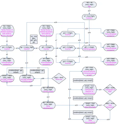
3.2. Achondroplasia

In the Achondroplasia KB [Nussbaum, McInnes, and Willard, 2001], the proband was

referred to the clinic since he had typical physical features of achondroplasia3 at birth.

Neither the parents nor the three paternal half-siblings of the proband showed any signs of

achondroplasia. There was also no family history of this autosomal dominant disease on

either the mother‟s or father‟s side. The clinic suspected that the father may have developed a

newly mutated gene which in turn was transmitted to the child. This was based on the fact

that the father was 45 years old. Studies show that the fathers of children affected with

achondroplasia tend to be older than the population mean for fathers at the time of

conception of the child [Korf, 2000]. A high rate of mutation is found in the male population

aged 35 and above, whereas no such effect is seen on the female counterpart. A DNA test as

well as a radiograph and a fetal ultrasound were recommended. Figure 3-4 shows the KB at

this state.

3

(34)

hm = false (very_high) 'family history of skeletal dysplasia,

birth defects, genetic disorders'

gm = 0 (high) 'FGFR3'

sm = false (very_high) 'Achondroplasia

symptoms'

hf1 = false (very_high) 'family history of skeletal dysplasia,

gf1 = 0 (high) 'FGFR3'

sf = false (very_high) 'Achondroplasia

symptoms' gp = 1 (high)

'FGFR3'

gf2 = 1 (high) 'FGFR3 germline' gs1 = 0 high)

'FGFR3'

gs2 = 0 (high) 'FGFR3'

ss1 = false (very_high) 'Achondroplasia

symptoms'

ss3 = false (very_high) 'Achondroplasia symptoms' a1 a5 a3 a2 a4 a6 a9 a8 a7 a20 a21 a22 a23 a24 a25 a19

bp = abnormal (high) 'FGFR3 protein'

pp = abnormal (high) 'bone development'

ef = true (high) 'mutation' hf2 = 45 (very_high) ‘age’ a11 a12 a27 a26

sp1 = true (very_high) 'physical features of Achondroplasia at birth' a13 tstp1 = recommended 'DNA test' tstp2 = recommended 'radiograph at birth' tstp3 = recommended 'fetal ultrasound' xor_resp ([gm, gf1, gf2], gp)

Figure 3-4: The pretest state of the Achondroplasia KB.

The DNA test revealed both the G1138A and the G1138C mutations in the proband‟s FGFR3

(Fibroblast Growth Factor Receptor 3) gene. A positive result of the G1138A mutation

typically yields a 98% accuracy rate in the diagnosis of achondroplasia, whereas

approximately 1-2% of the patients testing positive for the G1138C mutation end up having

the disease [Nussbaum, McInnes, and Willard, 2001]. The radiograph test further confirmed

(35)

fetal rhizomelia (a disproportion in the length of the upper arms and thighs) and fetal

macrocephaly (an abnormal largeness of the head). Figure 3-5 illustrates the KB at this state.

symptoms'

symptoms' gp = 1 (very_high)

'FGFR3'

symptoms'

bp = abnormal (very_high) 'FGFR3 protein'

pp = abnormal (very_high)

'bone development'

ef = true (high) 'mutation' hf2 = 45 (very_high) ‘age’ a10 a12 a27 a26

sp1 = true (very_high) 'physical features of Achondroplasia

at birth'

tresp2 = true (very_high)

'fetal macrocephaly' tresp5 = true

(very_high) 'radiographic

features of Achondroplasia'

tresp1 = true (very_high) 'fetal rhizomelia'

a18 a16

a17 tresp3 = true

(very_high) 'G1138A mutation

in FGFR3 gene' tresp4 = false

(very_high) 'G1138C mutation

in FGFR3 gene'

a13 tstp1 = done

'DNA test'

tstp2 = done 'radiograph at

birth'

tstp3 = done 'fetal ultrasound' a14 a15 a45 a44 a28 a28 a29 enables([tstp1, gp], tresp3) enables([tstp1, gp], tresp4)

enables([tstp2, pp], tresp5)

enables([tstp3, pp], tresp2) xor_resp

([gm, gf1, gf2],

gp)

a11

Figure 3-5: The posttest state of the Achondroplasia KB.

The clinic further predicted that it is possible the proband will encounter complications in his

symptoms which may lead to sudden death during the first year of age. Studies show that the

(36)

[Nussbaum, McInnes, and Willard, 2001]. The counselor also recommended specific

treatments for complications during infancy and early childhood, as well as for complications

during later childhood and early adulthood. Figure 3-6 shows this future KB state.

symptoms'

symptoms' gp = 1 (very_high)

'FGFR3'

symptoms'

bp = abnormal (very_high) 'FGFR3 protein'

pp = abnormal (very_high)

'bone development'

ef = true (high) 'mutation' hf2 = 45 (very_high) ‘age’ a11 a10 a12 a27 a26

sp1 = true (very_high) 'physical features of Achondroplasia

at birth'

'fetal macrocephaly' tresp5 = true

(very_high) 'radiographic

features of Achondroplasia'

tresp1 = true (very_high) 'fetal rhizomelia'

a18 a16

a17 tresp3 = true

(very_high) 'G1138A mutation

in FGFR3 gene' tresp4 = false

(very_high) 'G1138C mutation

in FGFR3 gene'

a13 tstp1 = done

'DNA test'

tstp2 = done 'radiograph at

birth'

tstp3 = done 'fetal ultrasound' a14 a15 a45 a44 a28 a28

cp1 = true (high) 'complications in

first year' a30 cp2 = true (high)

'sudden death in first year'

a31

cp4 = true (high) 'complications during later childhood and early adulthood' a29 a33 cp3 = true (high)

'complications during infancy and

early childhood' a32 trtp2 = reocmmended 'unspecified-2' a35 trtp1 = reocmmended 'unspecified-1' a34 inhibits([trtp1, pp], cp3)

enables([tstp1, gp], tresp3) enables([tstp1, gp],

tresp4)

enables([tstp3, pp], tresp2) xor_resp

([gm, gf1, gf2],

gp)

inhibits([trtp2, pp], cp4)

(37)

3.3. Familial Hypercholesterolemia

hp1 = false (high)

'French Canadian ancestry'

hp2 = false (high)

'family history of CHD'

gp =1 (high)

'LDLR'

gc1 = 1 (high)

'LDLR'

gc2 = 1 (high)

'LDLR'

gc3 = 1 (high)

'LDLR'

bp = abnormal (high)

'elevated LDL'

bc1 = abnormal (high)

'elevated LDL'

bc2 = abnormal (high)

'elevated LDL'

bc3 = abnormal (high) 'elevated LDL' a1 a2 a19 a17 a18 a5 a20 a21 a22

sp = true (very_high)

'myocardial infarction'

bhp2 = true (very_high)

'smoker'

'mild obesity'

bhp3 = true (very_high) 'physical inactivity' a6 tstp1 = recommended 'gene test' tstp2 = recommended 'LDL test' tstc1 = recommended 'LDL test' tstc2 = recommended 'LDL test' tstc3 = recommended 'LDL test' enables([bhp1

, bp], sp) enables([bhp2, bp], sp)

enables([bhp3, bp], sp) a7

a8 a9

Figure 3-7: The pretest state of the Familial Hypercholesterolemia KB.

In the Familial Hypercholesterolemia KB [Nussbaum, McInnes, and Willard, 2001], the

proband was referred to the clinic after he experienced a symptom of myocardial infarction

(commonly known as a heart attack). The counselor initially diagnosed him with familial

hypercholesterolemia, a genetic disorder characterized by very high LDL (low-density

lipoprotein) cholesterol and early cardiovascular disease. Studies show that this autosomal

dominant disease is more prevalent in the French Canadian population. Even though the

proband has neither French-Canadian ancestry nor any family history of the disease, several

(38)

also suspected that all three offspring of the proband may have also inherited the disease.

Thus both a gene test and an LDL test were recommended for the proband himself and an

LDL test was recommended for all of his offspring. Figure 3-7 shows the relationships

between the concepts described at this state.

hp1 = false (high)

'French Canadian ancestry'

hp2 = false (high)

'family history of CHD'

gp =1 (very_high)

'LDLR'

gc1 = 1 (very_high)

'LDLR'

gc2 = 1 (very_high)

'LDLR'

gc3 = 0 (very_high)

'LDLR'

'elevated LDL'

'mutation in 1 allele'

bc1 = abnormal (very_high)

'elevated LDL'

bc2 = abnormal (very_high)

'elevated LDL'

bc3 = normal (very_high)

'elevated LDL'

tresc1 = true (very_high)

'LDL result'

tresc2 = true (very_high)

'LDL result'

tresc3 = false (very_high) 'LDL result' a1 a2 a15 a16 a19 a17 a18 a5 a20 a21 a22 a23 a26 a28 a4

sp = true (very_high)

'myocardial infarction'

'smoker'

'mild obesity'

bhp3 = true (very_high) 'physical inactivity' a10 a11 a12 a7 a9 a8 a6 a13

'LDL result'

a14 tstp1 = done

'gene test'

tstp2 = done

'LDL test' tstc1 = done 'LDL test' tstc2 = done 'LDL test' tstc3 = done 'LDL test' trtp1 = recommended 'weight loss'

trtp2 = recommended 'stop smoking' trtp3 = recommended 'exercise' trtp4 = recommended 'drug’ trtp5 = recommended 'low-cholesterol diet' a3 a24 a25 a27 enables([bhp1 , bp], sp)

enables([bhp2, bp], sp)

enables([bhp3, bp], sp) enables([tstp1, gp], tresp1)

enables([tstp2, gp], tresp1) enables([tstc1, bc1], tresc1)

enables([tstc2, bc2], tresc2)

enables([tstc3, bc3], tresc3)

(39)

The proband‟s gene test confirmed a mutation of the LDLR gene in one allele. The LDL test

also revealed an elevated level of LDL choresterol in the proband, as well as two out of three

of his offspring. Approximately 5% of the patients who have high LDL end up actually

having the disease [Nussbaum, McInnes, and Willard, 2001]. The counselor recommended a

drug treatment along with a low-cholesterol diet for the proband. At the same time, he was

encouraged to stop smoking, undergo a weight loss, and start exercise regularly. Figure 3-8

shows the KB at this state.

3.4. Phenylketonuria

gm = 1 (very_high)

'phenylalanine gene'

sm = false (very_high)

'PKU symptoms'

gp = 2 (very_high)

gf = 1 (very_high)

sf = false (very_high)

'PKU symptoms'

bp = toxic (very_high) 'phenylalanine substrate level' trtp1 = recommended 'low phenylalanine diet started early in

life'

tstp = done

'phenylalanine concentration'

tresp = true (very_high) 'phenylalanine concentration' a1 a2 a3 a4 a5

a8 a6 a7

enables([tstp, bp], tresp) joint_resp([gm, gf], gp)

Figure 3-9: The posttest state of the Phenylketonuria (PKU) KB.

In the Phenylketonuria (PKU) KB [Korf, 2000], the proband was initially referred to the

clinic for a phenylalanine concentration test following an abnormal result of a standard

newborn screening. The test result revealed an abnormally high phenylalanine level,

(40)

counselor believed both parents were carriers, each contributing one mutated gene to their

offspring, even though neither of them displayed any PKU symptoms. The counselor

recommended that a low phenylalanine diet be started for the proband. This is very

important, especially for the first few years of life during which brain development is taking

place. The KB at this state is depicted in Figure 3-9.

gm = 1 (very_high)

sm = false (very_high)

'PKU symptoms'

gp = 2 (very_high)

gf = 1 (very_high)

sf = false (very_high)

'PKU symptoms'

bp = toxic (very_high) 'phenylalanine substrate level' trtp1 = recommended 'low phenylalanine diet started early in

life'

tstp = done

'phenylalanine concentration'

tresp = true (very_high) 'phenylalanine concentration' a1 a2 a3 a4 a5

a8 a6 a7

bo = toxic (high)

'fetal phenylalanine

level'

po = true (high)

'damage to development of major organ systems'

trtp2 = recommended

'low phenylalanine diet started prior to

pregnancy'

pp = true (high)

'central nervous system damage'

sp = true (high)

'delayed cognitive development'

so2 = true (high)

'low birth weight'

so1 = true (high)

'congenital heart disease'

so3 = true (high)

'developmentally impaired' a9 a10 a11 a12 a13 a14 a15 a16

enables([tstp, bp], tresp) joint_resp([gm, gf], gp)

inhibits([trtp2, bp], bo)

(41)

In the future, the counselor believed the proband had a chance to experience damage to her

central nervous system, which in turns would lead to a delayed cognitive development.

Furthermore, the counselor also predicted that the proband was likely to give birth to an

offspring who would have been exposed to an abnormally high phenylalanine level in the

fetal environment, resulting in the damage to development of its major organ systems,

including the brain. It is common for such infant to have low birth weight, congenital heart

disease, and inadequate brain development at the time of birth. A low phenylalanine diet was

(42)

CHAPTER 4 DISCOURSE GRAMMAR

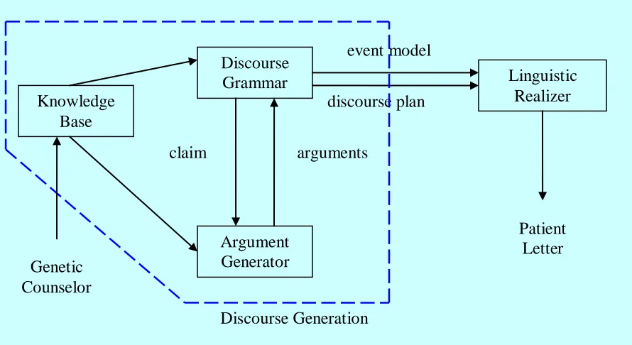
The discourse generation process used in GenIE involves three separate modules: a

qualitative causal probabilistic domain model, a genre-specific discourse grammar, and a

normative argument generator [Green, 2006]. The first component was discussed in Chapter

2. This chapter presents the second component – the discourse grammar. The final

component – the argument generator, will be discussed in detail in the next chapter.

Figure 4-1: The discourse generation process.

event model

Discourse Generation

discourse plan Knowledge

Base

Discourse Grammar

Argument Generator

Linguistic Realizer

Patient Letter

claim arguments

(43)

As illustrated in Figure 4-1 above, the discourse grammar extracts information from the

knowledge base to construct a claim. The claim is then passed on to the argument generator

which in turn returns a list of arguments that support the claim. An output of the DG is a

discourse plan that is later converted into an English text by the linguistic realizer.

Accompanying the discourse plan is an event model containing the event propositions

referred to by the discourse plan. The final English text output is the first draft of a patient

letter generated by GenIE.

4.1. Overview

The discourse grammar (DG) determines the organization of the patient letter to be

generated, initially as a generic outline and later instantiated with information specific to a

patient‟s case. The DG rules are based upon an analysis of the corpus done in a previous

study, [Green, 2006], as well as a description of standard practice in genetic counseling

[Baker et al., 2002]. The format of the DG output has been designed so that it can be easily turned into natural language sentences.

The DG generates a data structure called the discourse plan or dplan, a list of trees whose internal nodes specify discourse relations, and whose leaves specify propositions in the form

of events [Green, 2007]. Discourse relations are based upon a modified version of Mann and

Thompson‟s Rhetorical Structure Theory (RST) [Mann and Taboada, 2007], a theory of text

(44)

and text generation. Table 4-1 shows the list of nucleus-satellite RST relations used in the

DG, whereas Table 4-2 shows the list of multinuclear RST relations used.

Table 4-1: List of nucleus-satellite RST relations used in the Discourse Grammar.4

Relation Name Nucleus Satellite

Attribution A claim The person to whom a claim is

attributed

Background Text whose understanding is being

facilitated

Text for facilitating

understanding

Condition Action or situation whose occurrence

results from the occurrence of the

conditioning situation

Conditioning situation

Evaluation A situation An evaluative comment about

the situation

Evidence A claim Information intended to increase

the reader‟s belief in the claim

Purpose An intended situation The intent behind the situation

4

(45)

Table 4-2: List of multinuclear RST relations used in the Discourse Grammar.5

Relation Name Each Nucleus

Conjunction The items are conjoined to form a unit in which each item plays a

comparable role

Disjunction An item presents a (not necessarily exclusive) alternative for the other(s)

List An item comparable to others linked to it by the List relation

Narration6 Each argument is in temporal order

Event propositions are represented in the form of the four-place predicate:

event(ID, Modality, Semantics, Graph)

where ID uniquely identifies the event, Modality consists of a list of features that describe the event such as time, duration, polarity, probability, etc., Semantics describes the event in terms of its type of action and the semantic roles of the individuals involved in the action,

and Graph tells which KB state the event is based upon.

4.2. Discourse Plan

The starting rule of the DG generates four main sections of a patient letter in the form of a

discourse plan or dplan. Figure 4-2 below shows a rough organization of the dplan. The four main sections of the dplan are

5

The first three relations were extracted from a complete list in [Mann and Taboada, 2007]. 6

(46)

Preliminary diagnosis: doc_pretest

Final diagnosis: doc_diagnosis

Origin of genetic condition: doc_source

Future risk: doc_sibling_risk

dplan

doc_pretest doc_diagnosis doc_source doc_sibling_risk

narration

referral_event pretest_diagnosis testing test_result retract_initial_diagnosis

Figure 4-2: A rough organization of the dplan.

The four sections together form an initial outline of the information to be presented in the

letter, including various claims that require an argument to support their validity. Each of the

claims is then passed to the argument generator described in the next chapter. The

information returned by the argument generator is added to the initial outline, thus

completing the structure that will later be transformed by the linguistic realizer into English

(47)

The first section, doc_pretest, narrates the events involving the referral event that brought the proband to the clinic leading to a preliminary diagnosis of what genotype(s) caused the

symptoms. The DG consults the KB to get specific information on the list of symptoms the

proband was experiencing as well as the list of genotypes the proband was suspected of

having, then constructs the claim that the said genotype was responsible for the said

symptom(s). Also provided is the list of tests that had been done on the proband, together

with corresponding test results. The final optional subsection handles the case when the

preliminary diagnosis has been disconfirmed by the test results.

The second section of the letter, doc_diagnosis, presents the final diagnosis following the testing done on the proband. This posttest diagnosis is later backed up by the results of

specific tests done on the proband when the DG invokes the argument generator to get

arguments to support the claim.

The third section, doc_source, describes the source of the proband‟s genotype. The structure varies depending whether the disease of interest is an autosomal recessive or autosomal

dominant disorder. For an autosomal recessive case, information on both parents is included,

whereas for an autosomal dominant case, only the information relevant to the carrier is

(48)

The fourth section, doc_sibling_risk, provides information on potential risk of disease inheritance for the proband‟s future siblings. The risk is presented in terms of the probability

that a future offspring of the same pair of parents may inherit the same disease.

In the case where no particular information is available, the entire section will be replaced

with a null clause ([] – an empty list in Prolog), indicating that such detail is to be ignored

during English text generation. With it being the most important piece of information, the

second section, doc_diagnosis, is the only section that is required in the dplan. Without a proper diagnosis, there would be no reason for a patient letter to be generated in the first

place. Detailed examples of dplans for the four KBs covered in this thesis are shown in the appendix section.

Each of the DG rules used to construct the dplan consists of one or more nonterminals and/or predicates provided in the KB‟s Application Program Interface (API). The predicates are

used to access specific details in the KB that are to be included in the content of the patient

letter. For example, the predicate get_symptoms_set(Graph, Who, SymptomList) returns a list of symptoms the person Who was experiencing at the time of Graph (pretest, posttest, or future). Similarly, get_genotype_set, get_test_set, and get_test_result_set, each return a list of mutated genes, tests, and test results for the requested person and time, respectively.

Once information is obtained from the KB through the APIs, corresponding event

(49)

turns supplies arguments that support the claim. The next chapter describes the process of

(50)

CHAPTER 5 ARGUMENT GENERATION

The argument generator (AG) generates arguments for the claims passed to it from the DG,

using non-domain-specific argument strategies [Green, 2006]. The arguments justify the

conclusions of the genetic counselor about the patient‟s case. The following sections explain

first the layout of arguments according to Toulmin‟s model and then the argument schemes

used in GenIE. The last section presents some implementation details of the AG.

5.1. Elements of Arguments

According to Toulmin‟s model of argument structure [Toulmin, 2003], every acceptable

argument shares the same layout of basic elements, consisting of six interrelated components,

as listed in Table 5-1 below.

Table 5-1: The six elements of argument in Toulmin’s argument structure [Toulmin, 2003].

Element of Argument Definition

Claim The assertion that is to be established

Data The evidence supporting the claim

Warrant The reasoning that justifies the claim

(51)

Table 5-1(continued).

Element of Argument Definition

Rebuttal The condition that undermines the warrant or the backing

Qualifier The degree of certainty expressed for the claim

In GenIE, argument strategies map formal properties of the domain model to the data and

warrant supporting a claim and to the backing of a warrant [Green, 2006]. The next section

describes the different argument schemes. Each argument is translated into an RST tree

format after it is generated before adding it to the dplan. Figure 5-1 illustrates the RST representation of an argument [Green, 2007].

Figure 5-1: The RST representation of an argument [Green, 2007].

5.2. Argument Schemes

An analysis of the corpus done in a previous study in [Green, 2006] resulted in seven

different argument strategies to cover the argument generation needed for our domain. All of

the arguments generated for each sample KB were constructed using one or more of these n

s n s

background

warrant evidence

data claim

(52)

seven argument schemes. A number of arguments were formed as sequences of arguments.

An example of such complex arguments is elaborated in Section 5.3. Let us first look at each

of the seven argument schemes in detail.

Argument Scheme: E2C (Effect to Cause)

Claim: A ≥ VA

Data: B ≥ VB

Warrant: S+ ([A, VA], [B, VB])

Applicability Constraint: ¬ ( CX– ([[C, VC], [A, VA]], [B, VB]), C ≥ VC)

Figure 5-2: The applicability constraint of the E2C argument scheme.

The Effect-to-Cause argument scheme justifies a belief in a claim based on a possible causal

effect. In this strategy, the claim that the value of A has reached its threshold value VA is

supported by the data that the value of B has reached its threshold value VB. The warrant is

S+ ([A, VA], [B, VB]), i.e., that the state [A, VA] could be responsible for the state[B, VB]. An

S+

X– A

Argument Generation for a Biomedical Domain

-BIOGRAPHY

TABLE OF CONTENTS

LIST OF TABLES

LIST OF FIGURES

CHAPTER 1

INTRODUCTION

1.1. Genetics Background

1.2. Related Work

1.3. Thesis Organization

CHAPTER 2

DOMAIN MODEL

2.1. Qualitative Probabilistic Network

2.2. Implementation

2.3. Qualitative Relations

CHAPTER 3

OVERVIEW OF KNOWLEDGE BASES

3.1. Cystic Fibrosis

3.2. Achondroplasia

3.3. Familial Hypercholesterolemia

3.4. Phenylketonuria

CHAPTER 4

DISCOURSE GRAMMAR

4.1. Overview

4.2. Discourse Plan

CHAPTER 5

ARGUMENT GENERATION

5.1. Elements of Arguments

5.2. Argument Schemes