Computational study of decaying annular vortex flow using the r ε/k-ε turbulence model

(1)

Computational study of decaying annular vortex ﬂow using the

R

_e

/

k

e

turbulence model

Khalid M. Saqr

a,c,⇑

, Hassan I. Kassem

a

, Hossam S. Aly

b

, Mazlan A. Wahid

a a

High-Speed Reacting Flow Laboratory, Faculty of Mechanical Engineering, Universiti Teknologi Malaysia, 81310 Skudai, Johor Bahru, Malaysia

b

Department of Physics and Astronomy, University of Leicester, University Road, Leicester LE1 7RH, United Kingdom

c

Department of Aeronautical Engineering, Faculty of Engineering, King Abdulaziz University, Jeddah 21589, Saudi Arabia

a r t i c l e

i n f o

Article history:

Received 20 September 2010

Received in revised form 20 November 2011 Accepted 27 November 2011

Available online 3 December 2011

Keywords:

Vortex ﬂow Decaying vortex OpenFOAMÒ

Turbulence modeling CFD

a b s t r a c t

In this article, we present three dimensional CFD study of turbulent vortex flow in an annu-lar passage using OpenFOAM 1.6. The vortex flow is generated by introducing the flow through a tangential entry to the passage. For the analysis presented in this article, turbu-lence was modeled using theRe/kemodel, in addition, a comparison between such model with the standardkemodel was conducted and discussed. The main characteris-tics of the flow such as vortex structure and recirculation zone were investigated. It was found that flow is subjected to Rankine vortex structure with three forced vortex regimes and a free vortex region near to the outer wall. The phenomenon of vortex decay was inves-tigated by depicting the swirl number trend along the axial direction of the flow domain. It was found that the vortex decay is subjected to an exponential decay behavior. New coef-ficients for the exponential decay correlation were derived based on local values of velocity components in different radial planes.

1. Problem description

Vortex flow in annular passages can be found in several industrial equipments such as gas turbines[1–3], gas–solid cyclone separators[4–6]and heat exchangers[7,8]. Comprehending the major mean flow phenomena, such as recirculation zones and vortex decay, is crucial for the design and operation of such equipments. A major theoretical limitation, in the problem of turbulent vortex flow, is the insufficient information about the interaction between the different vortex regimes and largely varying turbulence scales[9–13]. Although there is a traditional consensus which dictates that forced vortex regime stabilizes (i.e. suppresses) turbulence and free vortex regime destabilizes (i.e. promotes) turbulence[14,15], more detailed phenomena such as the interaction between recirculation zone and turbulence, vortex core stretching, the com-mencement of the recirculation zone and the vortex core precession are not fully understood.

When the vortex flow is imparted into an annular passage, an increased level of complexity becomes evident. A new layer of near-wall shear flow is added, in such case, compared to the vortex flow in a cylindrical passage. Therefore, the behavior of the recirculation zone, vortex breakdown bubble and the vortex core become fundamentally distinct from such of the cylin-drical vortex flow. This distinction is also applied to the structure, velocity pattern and decay rate of vortex and turbulence intensity. Therefore, annular vortex flow can be deemed to be a different flow phenomenon than cylindrical vortex flow. In

⇑ Corresponding author at: High-Speed Reacting Flow Laboratory, Faculty of Mechanical Engineering, Universiti Teknologi Malaysia, 81310 Skudai, Johor Bahru, Malaysia. Tel.: +60 7 5534828; fax: +60 7 5566159.

E-mail addresses:[email protected],[email protected](K.M. Saqr).

Applied Mathematical Modelling 36 (2012) 4652–4664

Contents lists available atSciVerse ScienceDirect

Applied Mathematical Modelling

(2)

order to highlight the relevance of the present work, a brief review of the major efforts of describing annular vortex ﬂow is presented.

In fact, there have been few experimental attempts of describing the different regimes of annular vortex flows over the last four decades[16–20]. Vanierschot and Bulck[21]examined the effect of swirl on the cold flow field of an annular jet with a stepped-conical expansion using Laser Doppler Anemometry (LDA). They were able to identify four different annular jet regimes as a function of the swirl number. The same methodology was used by Sheen et al.[22]to observe the flow pat-tern and vortex breakdown phenomenon in unconfined annular swirling flow. These experimental efforts have added sub-stantial knowledge to the state of the art understanding of annular vortex flow. However, they did not successfully provide a universal theory for the major flow phenomena that occurs at different Reynolds numbers and swirl intensities.

The computational efforts to study annular vortex flow are rather few as well. Xicheng and Zhengming[23]have used an algebraic turbulence model to study the three dimensional viscous flow in an annular cascade with tip clearance. The objec-tive of their study was to determine the locations and structure of the leakage at the tip clearances. Garcia-Villalba and Frih-lich[24]have studied unconfined annular swirling flow at different swirl numbers using large eddy simulation (LES). They were able to provide an analysis of the impact of swirl on the mean flow and the precessing vortex structures. Similar tech-nique, assisted with PIV measurements, was used by Loureiro et al.[25]to investigate the characteristics of the flow field inside an annular space formed by two concentric cylinders with rotation of the inner cylinder. Such case is fundamentally different from the case presented in this paper since the vortex motion is imparted along the full length of the annulus, rather than through a single finite port such as the case in hand. There have been an interesting set of studies on the indus-trial application of vortex flow in cylindrical passages in gas–liquid separators by Ahmed et al. in the past few years. They have proposed a modified Eulerian–Lagrangian approach that is able to enhance the numerical prediction of separation pro-cess in[26]. From their results, it is evident that the new approach captures the effect of the vortex field on the separation efficiency more accurately than previous formulations. In some other recent studies from their group, the numerical mod-eling of high gas content gas–liquid vortex separators has been evaluated[27,28].

There are three major objectives for the present article. The ﬁrst is to extend the validity of theRe/k

e

turbulence model

in analyzing annular vortex ﬂows. The second objective is to compare the performance of such model with the standardk

e

model. The third objective is to shed the light on the vortex and turbulence decay phenomena that takes place in annular vortex ﬂows with large length to diameter aspect ratios, which has not been fully covered in literature, as it was shown ear-lier in this section. The turbulence model implementation in OpenFOAMÒ_{is described, and then the computational model} results are validated through several comparisons with the PIV local velocity measurements available from Ref.[29]. A com-parison between the result of theRe/k

e

model and such of the standardk

e

model is conducted to demonstrate the

prev-alence of theRe/k

e

model in the present ﬂow conﬁguration. Afterwards, the simulation results of a case with Re value of

5.4104_{are presented and discussed. In the present ﬂow conﬁguration, the inlet swirling strength depends on the inlet}

Rey-nolds number since the ﬂow is introduced to the passage with tangential velocity component only. The parameters of major concern herein are the vortex structure, swirl intensity, turbulence intensity and dissipation rate of turbulence kinetic en-ergy. These parameters are discussed with respect to their spatial distributions along the axial and radial dimensions of the annular passage.

2. Physical and mathematical formulation

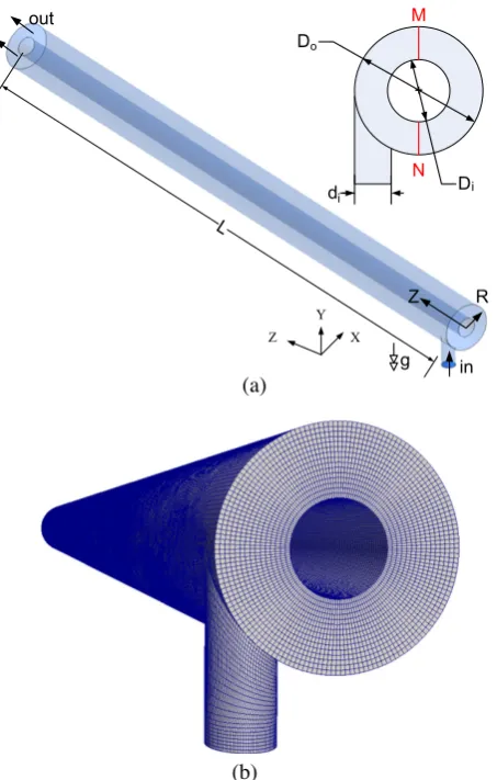
The case considered in this article is similar to the PIV measurement setup reported in[29]. The case selection was based on the availability of reliable experimental data for the purpose of validation and the adequacy of the case to represent the physics of annular decaying vortex flow. The flow domain is illustrated inFig. 1. Flow is introduced to the annular cylindrical passage through a tangential inlet pipe with a diameterdi. The inlet flow direction is reverse to the positive direction of the

gravity vector~g. The diameter of the inlet pipediis equal to the annular gap width, which is equal to half the difference

be-tween the annular passage’s outer and inner diameters. The ratio bebe-tween the passage length and outer diameter L Do equals to 30. The detailed dimensions and flow configurations are explained in[29]. According to[29], the measurement planes are vertical with respect to the direction of the gravity vector, and denoted by (M) and (N) as inFig. 1. The outlet flow direction is coaxial with the annular passage.

The flow configuration inFig. 1can be represented by the Reynolds averaged Navier Stokes equations for turbulent incompressible flow, in Cartesian coordinates as following:

Continuity equation:@uj @xj

¼0; ð1Þ

Momentum equation:

q

Uj @Ui

@xj ¼ @P @xiþ

@ @xj

tij

q

u0iu0j

; ð2Þ

wheretijis the viscous stress tensor deﬁned as

tij¼2

l

sij; ð3Þ

(3)

TheRe/k

e

turbulence model[30,31]can be given by the equations of turbulence kinetic energykand its dissipation rate

e

, respectively:

q

uj @k @xj¼

s

ij @_u_j @xi

qe

þ @

@xj

l

þ

l

T

r

k

_@

_e

@xj

; ð4Þ

whereUiis the mean velocity,

s

ijis the Reynolds stress tensor,xiis the position vector,

l

Tis the eddy viscosity,

r

kis a closure

coefﬁcient that has a unity value, and

e

is the dissipation rate.

q

uj @

e

@xj

¼Ce1

e

k

s

ij

@uj @xj

Ce2

q

e

2

kþ @ @xj

l

þ

l

T

r

e

_@

_e

@xj

m

TS

3

ð1

g

=

g

0Þ

1þb

g

3 ; ð5Þ

where

g

¼Sk=

e

; ð6Þ

and S¼ ð2SijSijÞ1

=2

: ð7Þ

Sijis the mean rate of strain tensor,

g

04.38 andb= 0.012. The turbulence viscosity is expressed as

l

T¼

q

Cl

k2

e

: ð8Þ

The model constantsCe1,Ce2,Cland

re

values are 1.44, 1.92, 0.09 and 1.3, respectively, as reported in[32,33].

(a)

(b)

Fig. 1.(a) Schematic of the ﬂow domain and three dimensional orientation, (b) a 3D screenshot of the discretized computational domain as shown on ParaView 3.6.

(4)

3. Computational methodology

The numerical simulations reported in the present work have been conducted using OpenFOAMÒ_{1.6.x code. OpenFOAM}Ò has attracted much attention recently because it is a sustainable open source code designed for a wide range of CFD applications. It is a C++ toolbox based on object oriented programming [34]. OpenFOAMÒ _{is released under the GPL} [35,36]and it consists of enormous groups of libraries for different mathematical, numerical and physical models. Linking the mathematical/numerical tools with the physical models in a main C++ function produces different solvers and utilities. TheRe/k

e

turbulence model has been coded and compiled in the OpenFOAMÒcode. The simulations reported herein were

conducted using the SimpleFoam solver of OpenFOAMÒ_{. This solver is a steady-state solver for incompressible turbulent} ﬂow. OpenFOAMÒ_{allows the users to freely choose among a wide range of for numerical discretization and interpolation} schemes. The numerical schemes used in the SimpleFoam solver in the present study are listed inTable 1.

3.1. Solver parameters

3.1.1. The SimpleFoam solver

SimpleFoam is a pressure-based solver which solves the momentum equation with under relaxation factors and then iter-atively applies a pressure corrector equation based on the conservation of mass to evaluate the velocity and pressure fields. The turbulence model equations are solved after the velocity and pressure fields are computed for each step, and an iterative update is performed on the latter fields before a consecutive step is performed. In the present work, the under-relaxation factors were had values as listed inTable 1.

3.1.2. Convergence criteria

The convergence criteria for all cases were set to residuals value of 105_{for the pressure field and 10}6_{for other flow field}

variables. Residuals are measures of the error in the solution so that the smaller they are, the more accurate the solution. More precisely, the residual is evaluated by substituting the current solution into the equation and taking the magnitude of the difference between the left and right hand sides; it is also normalized in to make it independent of the scale of problem being analyzed[37].

3.1.3. Mesh non-orthogonality

Another important solver parameter is the non-orthogonality correction. Non-orthogonality represents a measure of mesh quality and it is deﬁned as the angle between the vector which joins two cell centroids and the normal vector for common face in-between such cells. The importance to have non-orthogonality minimized arises when one considers that in the ﬁnite vol-ume method volvol-ume integrals of spatial derivatives are converted to surface integrals and then such surface integrals are approximated over cell faces, with the latter approximation involves interpolation from cell centers to faces. In OpenFOAM, a correction scheme is available to take into account the effect of local mesh non-orthogonality on the interpolation required to evaluate cell face gradients. We have conducted several exercises on the grids used in the present article and found out that such grids required two iterations of such correction scheme to eliminate the effect of local mesh non-orthogonality.

3.1.4. The SIMPLE algorithm

The Semi-Implicit Method of Pressure Linked Equations (SIMPLE)[38]is the algorithm by which the governing equations are solved in SimpleFoam solver. This algorithm solves the momentum matrix and then applies a pressure correction to con-serve the incompressibility constraint implied by the continuity equation. This process is iterative. Within the main iteration conducted by the SIMPLE algorithm there is a momentum corrector step conducted to ensure that the velocity ﬁeld is up-dated according to the new pressure values. In the present work, such momentum corrector step was conducted twice for each iteration in all cases. This was necessary to reach the convergence criterion for the pressure ﬁeld.

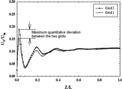
3.2. Grid independency and near-wall treatment

The computational grids were created using the commercial discretization software GambitÒ_{2.3, and then converted to} OpenFOAMÒ _{grid using the ﬂuentMeshToFoam grid conversion tool. Two grids were tested to ensure that the results}

Table 1

List of numerical schemes and under-relaxation factors employed in SimpleFoam solver for the present study.

Terms Discretization scheme Interpolation scheme

Gradient (r) Second order Gaussian integration Second order – central differencing

Divergence (r) TVD limited linear differencing

Laplacian (r2₎ _{Second order – central differencing}

Under-relaxation factors

p U k e

(5)

obtained by the solver and the turbulence model are not dependent on the grid. The ﬁrst grid had 9.62105_{cells and the}

second grid has 3.45106_{cells. The normalized axial (Z) velocity proﬁles obtained by the two grids are compared in}_{Fig. 2}_.

There is no qualitative difference between the two solutions of the two grids. Only a minimum quantitative difference can be observed fromFig. 2. The maximum value of this quantitative difference is equal to 3% of the normalized axial velocity, as demonstrated inFig. 2. Thus, it can be concluded that the solver and numerical schemes implementation yield results that are independent from the grid.

The turbulence models used in the present work are all high-Re models. Hence, a wall function was necessary to model the ﬂow near to the wall. They+_{values for the problems solved herein had an average of 15.307 and minimum and}

maxi-mum values of 1.831 and 69.431, respectively. Along the inner wall of the annular passage, they+_{value did not exceed 25.68}

in all cases. ThenutWallFunctionwas used in the SimpleFoam solver. Such wall function applies the logarithmic law-of-the wall for mean velocity ﬁelds wheny+_{> 11.0 in SimpleFoam, as in Eq.}₍₉₎_{. The OpenFOAM user manual}_[37]_{and turbulence}

modeling texts may be consulted for the details of the logarithmic law-of-the wall.

Uþ¼1 ko

lnðyþ_{Þ þ}_N; _ð9Þ

whereU+is the local velocity normalized by the frictional velocity at the nearest wall,kois the Von Karman’s constant (0.4)

andNis a numerical constant equals to 5.14.

4. Results and discussion

4.1. Experimental validation and turbulence models comparison

4.1.1. Boundary conditions

TheRe/k

e

turbulence model has been recently validated in[30,31,39]for different conﬁgurations of ﬂows that are

dom-inated by forced vortex fields. Further validation of the model is presented in this section. The case study was adopted to validate the model and code for the flow configuration presented in[29], which has the same flow configuration as in Fig. 1. The Reynolds number of the flow was 5400, for the validation case, based on the following expression[29]:

Re¼2eU

m

; ð10Þ

whereeis the annular gap width,Uis the average axial velocity calculated based on a water volumetric ﬂow rate of 2.14 m3_/

h and

m

is the kinematic viscosity. The Reynolds number value reported in[29], which was used for validation in the present article (Section 4.1.2), produced a vortex field that can be generally described as weak. Industrial applications utilizing vortex flow usually involve strong vortex fields that has high Reynolds number. Therefore in the results presented in Sections 4.3 and 4.4 the value of Re was increased one order of magnitude to become 54000.

4.1.2. Comparison of turbulence models

Turbulence modeling in swirling flow exhibiting vortex breakdown and recirculation resembles a significant challenge for industrial CFD approaches. Filtering approaches such as LES and DES are capable of capturing most of the details of such flow, however they require substantial computational resources which make them unsuitable for industrial applications[40]. Two equations turbulence models as well as the Reynolds stress model are the most commonly used turbulence models in

(6)

swirling ﬂow problems. Numerous recent researches provide evidences that such models are capable of predicting swirling ﬂows under vortex breakdown and recirculation[41–47]mainly using variants of the of thek

e

model. However, in regions where forced vortex ﬁelds are strong and dominant, different variants of thek

e

model produce ill predictions of the vortex ﬁeld. This has been addressed along the past three decades by introducing source term corrections in the

e

equation[48]to take into account the effect of streamline curvature due to ﬂow rotation. TheRe/k

e

turbulence model introduces a source

term in the

e

equation as well, but to express the local anisotropy assumption which is crucial for modeling strongly sheared ﬂows as postulated in[49,50]. The evaluation of this term and its integration in the

e

equation is given in Section 2. The mod-el has been successfully used to modmod-el unconfined swirling flow in Sydney burner[51]and shear driven vortex flow[31]and tornado-like vortex flow[52].

Figs. 3 and 4show a comparison between the vortex ﬂow ﬁeld as predicted by the standardk

e

model andRe/k

e

against experimental measurements. The axial velocity predictions of the two models are close, and both models over-pre-dict the axial velocity near to the outer wall. This can be attributed to the complexity of the ﬂow near to the wall, and also to the unsteadiness of the vortex breakdown region where the measurements plotted inFigs. 3 and 4were conducted. Such region exhibits a sharp drop in the vortex strength, as it is shown later in this article. The standardk

e

model, however, fails to predict the vortex motion compared to theRe/k

e

model as shown inFig. 4. The additional term in the

e

equation

of theRe/k

e

model damps the dissipation rate predictions by the standard model, in order to take into account the effect of

elevated strain rates produced by anisotropic turbulence inherited by swirling flows. This produces enhanced predictions of the forced vortex field, which complies with the theory of postulates that forced vortex regime produces a stabilizing effect on the turbulence field[53,54].

4.2. Vortex structure

The following results are based on Re = 54000. The vortex structure can be characterized by the spatial distribution of the tangential velocity. In the present ﬂow, the vortex structure exhibits signiﬁcant asymmetric behavior with respect to the

(7)

radial and axial distributions of tangential velocity component. Such asymmetric behavior is shown by depicting the con-tours of tangential velocity at different axial locations from the tangential inlet of the annular passage, as shown inFig. 5. The contour plots ofFig. 5clearly show the asymmetry of the vortex structure.

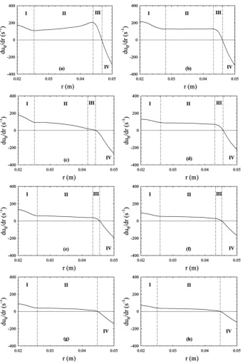
Another signiﬁcant parameter for characterizing the vortex structure is the radial derivative of tangential velocity duh dr .

Such parameter is important in identifying the regions dominated by forced or free vortex structures.Fig. 6shows proﬁles of

Fig. 4.Predicted and measured tangential velocity proﬁles at an axial distance of (a) 260 mm and (b) 550 mm from the inlet plane. Re = 5400.

(8)

duh

dr on a radial line parallel to theXaxis at different axial locations. Since the solver uses the Cartesian coordinate system,

the following relation was used to calculate the tangential velocity component in Cartesian coordinate system:

uh¼

uyux yx

xþyx2

: ð11Þ

The vortex structures can be classiﬁed, with respect to the radial derivatives of the tangential velocity as it appear in Fig. 6, to several regions. All the regions where such parameter has a positive value exhibit forced vortex, while the negative

(9)

values indicate a free vortex structure. In addition, the profiles show that there are several regions of forced vortex, while there is only one region of free vortex near to the outer wall. Therefore, the flow in the annular passage has a Rankine vortex structure. It can be observed that the flow exhibits multiple forced vortex structures near to the tangential inlet, until an axial distance equivalent to 12Do. This is shown in regions I, II and III illustrated inFig. 6(a–f). Each of these forced vortex

structures has a different radial gradient for the tangential velocity. At further axial locations, the third forced vortex region; III, disappears and only two forced vortex regions remains. At all axial locations, only one region of free vortex exist, which is denoted by IV inFig. 6. This free vortex region decelerates the ﬂow near to the outer cylinder of the annular passage.

4.3. Central recirculation zone (CRZ)

A central recirculation zone was found to exist in the vicinity of the inner wall of the annular passage. A coaxial planer velocity vector plot, surface and planer contour plots are shown inFig. 7. From such ﬁgure, it can be seen that the CRZ is

Fig. 7.(a) Surface plot of the stagnation axial velocity. The inset Fig. shows a front view of the annular passage. (b) planar plot of the velocity vector ﬁeld on a symmetricYZplane (c) monochrome contour plot of the recirculation zone on a symmetricYZplane.

(10)

highly asymmetric, and it can also be noticed that it is concentrated in the lower region of the passage, as shown in the inset ﬁgure. Similar asymmetric behavior of the CRZ was reported in[26]. The maximum length of the CRZ is 0.31 m. The total length of the measured CRZ in[26]was 0.365 m, thus the simulation underpredicts the CRZ length by 15%.

4.4. Decay of swirl intensity

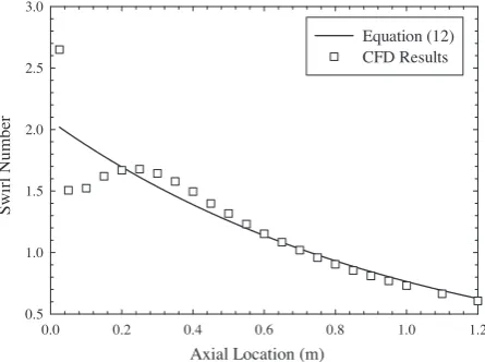
Swirl number is an efficient parameter to estimate the swirl intensity and its decay rate[55–57]. There is no universal mathematical definition for the swirl number; however, it can be physically defined as the ratio of the axial flux of the angu-lar momentum to the axial thrust[58,59]. In the present work, the swirl number is expressed as:

Sn¼

RRo Ri uzuhr2dr 2ðRoRiÞR

Ro Ri u2zrdr

: ð12Þ

The latter definition of the swirl number matches the definition proposed in[29]. The decay of swirl number in confined swirling flows can be qualitatively correlated by empirical correlations that usually take the form of exponential functions of the axial location along the pipe[60–62]. As shown in Eq.(12), the swirl number can be only calculated at a specific radial plane, by integrating over all the circumferential locations. Near to the inlet of the passage, where the flow is majorly sub-jected to tangential momentum, the swirl number should exhibit large values, compared to the values downstream the pas-sage. Pruvost et al.[29]provided the following general form for the empirical correlation to express the swirling decay in an annular passage:

dðSnÞ ¼aexp bz 2ðRoRiÞ

; ð13Þ

whered(Sn) is the local value of swirl number at a speciﬁc axial location (z). This correlation, of course, is dependent on the

Reynolds number and the geometry of the annular passage. The constants (a) and (b) were calculated to be 1.98 and 0.033, respectively, for a Re value of 5400 and a geometry similar to the one considered herein[29]. However, in the latter work, the swirl number was obtained at every axial location using only two angular locations. This means that a quasi-axisymmetric distribution for the tangential velocity component was assumed, when calculating the swirl number from the PIV data. Such assumption resulted in large deviations between the values of the measured and the predicted swirl decay, as reported in [29]. In another related research, Aouabed et al.[63]reported two values for the constant (b) for two different Reynolds num-ber, while they found that the constant (a) should be corresponding to the inlet swirl number, thus, depends only on the geometry. They concluded that the constant (b) decreases with the increase of Re. The parameter (a) is very sensitive to the initial swirl intensity. Therefore, in the case of tangential ﬂow entry, such as the one in hand, it becomes extremely dif-ﬁcult to separate the effects of Re and initial swirl intensity on the parameters (a) and (b).

The swirl number was computed at different axial locations along the annular passage and plotted inFig. 8at Re = 5400. This was done by performing the integrations of Eq.(12)on different surfaces in theXYplane (i.e. radial plane) which was not possible to be performed based on the experimental measurements. Therefore, in such computations, there is no assumption of axisymmetric distribution of the tangential velocity. In other words, the predicted swirl number using Eq. (12)was based on the local value of axial and tangential velocity component at every grid cell, on each speciﬁc radial plane. Statistical regression was used to obtain the constants (a) and (b) from such data, and were found to be 2.11 and 0.059,

Axial Location (m)

0.0 0.2 0.4 0.6 0.8 1.0 1.2

Sw

ir

l Nu

mb

er

0.5 1.0 1.5 2.0 2.5 3.0

Equation (12) CFD Results

(11)

respectively. The swirling decay predicted using Eq.(13)and the latter constant values is also plotted inFig. 8in comparison with the computed values from the CFD results.

Fig. 9shows a comparison between the measured and predicted swirl numbers based on the work of Pruvost et al.[29]. The values of (a) and (b) used in Eq.(13)for the predictions inFig. 9are 1.98 and 0.033, respectively, as obtained in their work. The difference between the predicted and measured values is quite large at approximately all the axial locations, as mentioned above. This large difference is due to the fact that only two angular planes were used for the swirl number cal-culations, on the contrary from the present work, where the swirl number was locally calculated based on the local value of velocity component at each grid cell.

5. Concluding remarks

TheRe/k

e

turbulence model has been successfully coded in a dynamic library in the open source CFD code OpenFOAM

1.6. A comparison between such model and the standardk

e

model showed its prevalence in predicting forced vortex ﬂows. Two simulations of decaying vortex ﬂow in an annular passage were successfully conducted usingRe/k

e

turbulence

model. The ﬁrst simulation (Re = 5.4103_{) was used to validate the turbulence model through comparison with previously}

reported PIV measurements and to derive new coefficients for the swirling decay correlation. The second simulation which was conducted at Re = 5.4104, was used to shed some light on the physics of the vortex flow field and swirling intensity decay in the annular passage. The following notes were concluded from analyzing the results:

1. The vortex ﬂow ﬁeld within the annular passage was found to be strongly asymmetric with respect to the radial distri-bution of tangential velocity component.

2. The vortex ﬂow ﬁeld within the annular passage contains more than one forced vortex region. The present case was found to have a maximum of three forced vortex regions, and a single free vortex region near to the outer wall.

3. A central recirculation zone was formed in the vicinity of the inner wall of the annular passage. The maximum length of the CRZ was found to be 0.31 m which deviates from the experimentally measured CRZ length by 15%.

4. The decay of swirling intensity was correlated using an exponential decay equation, and new values for the coefﬁcients of such equation were obtained.

References

[1] J. Becker, D. Heitz, C. Hassa, Spray dispersion in a counter-swirling double-annular air ﬂow at gas turbine conditions, Atomization Sprays 14 (1) (2004) 15–35.

[2] S. Bharani, S.N. Singh, D.P. Agrawal, Effect of swirl on the ﬂow characteristics in the outer annulus of a prototype reverse-ﬂow gas turbine combustor, Exp. Therm. Fluid Sci. 25 (6) (2001) 337–347.

[3] A. Ridluan, S. Eiamsa-ard, P. Promvonge, Numerical simulation of 3D turbulent isothermal ﬂow in a vortex combustor, Int. Commun. Heat Mass Transfer 34 (7) (2007) 860–869.

[4] H.W. Wang, J.J. Wang, Y.H. Jin, Numerical simulation of the gas phase ﬂow ﬁeld in inlet annular space of a guide vane cyclone tube, Petrochem. Equipment 35 (2) (2006) 33–36.

[5] L.Y. Hu, L.X. Zhou, J. Zhang, M.X. Shi, Studies on strongly swirling ﬂows in the full space of a volute cyclone separator, AIChE J. 51 (3) (2005) 740–749. [6] L. Hu, M. Shi, L. Zhou, J. Zhang, Numerical simulation of 3-D strongly swirling turbulent ﬂow in a cyclone separator, Qinghua Daxue Xuebao/J. Tsinghua

University 44 (11) (2004).

[7] E. Kavak Akpinar, Y. Bicer, C. Yildiz, D. Pehlivan, Heat transfer enhancements in a concentric double pipe exchanger equipped with swirl elements, Int. Commun. Heat Mass Transfer 31 (6) (2004) 857–868.

Axial Location (m)

0.0 0.2 0.4 0.6 0.8 1.0 1.2 1.4

Sw

ir

l Nu

mb

er

0 1 2 3 4 5

Swirl Number Calculated at Plane M Swirl Number Calculated at Plane N Equation (12)

(12)

[8] A. Durmusß, M. Esen, Investigation of heat transfer and pressure drop in a concentric heat exchanger with snail entrance, Appl. Therm. Eng. 22 (3) (2002) 321–332.

[9] M.T. Abujelala, T.W. Jackson, D.G. Lilley, SWIRL FLOW TURBULENCE MODELING, 1984. Cincinnati, OH, Engl: AIAA. [10] M.T. Abujelala, T.W. Jackson, D.G. Lilley, Swirl ﬂow turbulence modeling, 1984.

[11] S. Jakirlic´, K. Hanjalic´, C. Tropea, Modeling rotating and swirling turbulent ﬂows: a perpetual challenge, AIAA J. 40 (10) (2002) 1984–1996. [12] M. Baratta, A.E. Catania, S. d’Ambrosio, Nonlinear versus linear stress–strain relations in engine turbulence modeling under swirl and squish ﬂow

conditions, J. Eng. Gas Turbines Power 130 (6) (2008).

[13] S. Yapici, M.A. Patrick, A.A. Wragg, Hydrodynamics and mass transfer in decaying annular swirl ﬂow, Int. Commun. Heat Mass Transfer 21 (1) (1994) 41–51.

[14] P. Bradshaw, The analogy between streamline curvature and buoyancy in turbulent shear ﬂow, J. Fluid Mech. 36 (1969) 177–191. [15] P. Bradshaw, Effects of streamline curvature on turbulent ﬂow, AGARDograph AG-169, 1973.

[16] T.H. Chang, K.S. Lee, An experimental study on swirling ﬂow in a cylindrical annuli using the PIV technique, J. Visual. (2010) 1–9.

[17] D.L. Young, C.B. Liao, H.J. Sheen, Computations of recirculation zones of a conﬁned annular swirling ﬂow, Int. J. Numer. Methods Fluids 29 (7) (1999) 791–810.

[18] A. Hagiwara, S. Bortz, Near-ﬁeld aerodynamics of swirl burners (Part 3. Isothermal annular swirling ﬂows with and without primary air injection), Nippon Kikai Gakkai Ronbunshu, B Hen/Trans. Jpn. Soc. Mech. Eng. B 55 (511) (1989) 865–870.

[19] M.P. Escudier, Observations of the oscillatory behavior of a conﬁned ring vortex, AIAA J. 17 (3) (1979) 253–260. [20] C.J. Scott, D.R. Rask, Turbulent viscosities for swirling ﬂow in a stationary annulus, 1973.

[21] M. Vanierschot, E. Van den Bulck, Hysteresis in ﬂow patterns in annular swirling jets, Exp. Therm. Fluid Sci. 31 (6) (2007) 513–524.

[22] H.J. Sheen, W.J. Chen, S.Y. Jeng, Observations of flow pattern and vortex breakdown of an unconfined annular swirling jet flow, J. Chinese Soc. Mech. Eng. Trans. Chinese Inst. Eng. C 16 (3) (1995) 293–304 (Chung-Kuo Chi Hsueh Kung Ch’eng Hsuebo Pao).

[23] J. Xicheng, W. Zhengming, Numerical simulation of three-dimensional viscous ﬂow in annular cascades including tip clearance, in: Proceedings of the 1st International Conference on Engineering Thermophysics (ICET ’99), 1999, Beijing.

[24] M. Garcia-Villalba, J. Frihlich, LES of a free annular swirling jet – Dependence of coherent structures on a pilot jet and the level of swirl, Int. J. Heat Fluid Flow 27 (5) (2006) 911–923.

[25] B.V. Loureiro, P.R.S. Mendes, L.F.A. Azevedo, Characterization of fluid flow and Taylor vortex onset in partially-obstructed annular space with inner cylinder rotation, in: Proceedings of the ASME Heat Transfer/Fluids Engineering Summer Conference 2004, HT/FED 2004. 2004. Charlotte, NC. [26] S. Ahmed, G.S. Soto, J. Naser, E. Nakagawa, A modified Eulerian–Lagrangian approach applied to a compact down-hole sub-sea gas–liquid separator,

Sep. Sci. Technol. 46 (4) (2011) 531–540.

[27] S. Ahmed, G. Sanchez Soto, C. Wong, E. Nakagawa, J. Naser, Effect of pressure and salinity on the performance of a gas-liquid separator – A preliminary study, Australian Petrol. Product. Explor. Assoc. J. 51 (2011) 603–612.

[28] S. Ahmed, M.N. Noui-Mehidi, J. Naser, G. Sanchez Soto, E. Nakagawa, Evaluation of numerical modelling for a compact down-hole subsea gas–liquid separator for high gas content, Australian Petrol. Product. Explor. Assoc. J. 49 (2009) 433–440.

[29] J. Pruvost, J. Legrand, P. Legentilhomme, L. Doubliez, Particle image velocimetry investigation of the flow-field of a 3D turbulent annular swirling decaying flow induced by means of a tangential inlet, Exp. Fluids 29 (3) (2000) 291–301.

[30] K.M. Saqr, H.S. Aly, M.A. Wahid, M.M. Sies, Numerical simulation of confined vortex flow using a modifiedketurbulence model, CFD Lett. 1 (2) (2009) 87–94.

[31] K.M. Saqr, H.S. Aly, H.I. Kassem, M.M. Sies, M.A. Wahid, Computations of shear driven vortex ﬂow in a cylindrical cavity using a modiﬁedke

turbulence model, Int. Commun. Heat Mass Transfer 37 (8) (2010) 1072–1077.

[32] B.E. Launder, D.B. Spalding, Lectures in Mathematical Models of Turbulence, Academic Press, London, England, 1972.

[33] B.E. Launder, D.B. Spalding, The numerical computation of turbulent ﬂows, Comput. Methods Appl. Mech. Eng. 3 (1974) 269–289.

[34] H.G.W.a.G. Tabor, H. Jasak, C. Fureby, A tensorial approach to computational continuum mechanics using object-oriented techniques, Comput. Phys. (6) (1998).

[35]http://www.openfoam.com.

[36] OpenFOAM, OpenFOAM user guide. 2010.

[37] OpenCFD, OpenFOAM: The Open Source CFD Toolbox – User Guide Version 1.7.1, 2010, OpenCFD Limited. [38] S.V. Patankar, Numerical heat transfer and ﬂuid ﬂow, 1980: Hemisphere Pub. Corp.

[39] H.I. Kassem, H.S. Aly, K.M. Saqr, M.M. Sies, M.A. Wahid, Performance of RANS turbulence models in predicting strained ﬂows in a curved duct, in: International Conference on Fluid Mechanics and Heat & Mass Transfer, 2010, WSEAS Press: Corfu Island, Greece. p. 78–83.

[40] K. Hanjalic, Will RANS survive LES? A view of perspectives, J. Fluids Eng. Trans. ASME 127 (5) (2005) 831–839.

[41] K.R. Menzies, An Evaluation of Turbulence Models for The Isothermal Flow in A Gas Turbine Combustion System, in: W. Rodi, (Ed.), Sixth International Symposium on Engineering Turbulence Modeling and Experiments, 2005, Sardinia, Italy.

[42] G. Hsiao, H. Mongia, Swirl Cup Modeling Part III: Grid Independent Solution with Different Turbulence Models, in: 41st Aerospace Sciences Meeting & Exhibit, 2003, AIAA, Reno, Nevada.

[43] A. Smirnov, A. Lipatnikov, J. Chomiak, Simulations of swirl-stabilized premixed combustion. in American Society of Mechanical Engineers, Pressure Vessels and Piping Division (Publication) PVP, 1998. San Diego, CA, USA, ASME.

[44] S.J. Tarr, G. Allen, A. Aroussi, S.J. Pickering, Interaction of swirling ﬂows from two adjacent coal burners, in: American Society of Mechanical Engineers, Fluids Engineering Division (Publication) FED, 1997, Vancouver, Can, ASME.

[45] Y.P. Li, Q. Zhang, F. Gu, Y.Q. Xu, Numerical study on the effect of reverse swirl of secondary air on ﬂue gas imbalance in large tangentially ﬁred boiler, Proceedings of the Chinese Society of Electrical Engineering 21 (9) (2001) 33–37 (Zhongguo Dianji Gongcheng Xuebao).

[46] U. Engdar, J. Klingmann, Investigation of two-equation turbulence models applied to a conﬁned axis-symmetric swirling ﬂow, in: American Society of Mechanical Engineers, Pressure Vessels and Piping Division (Publication) PVP, 2002, Vancouver, BC.

[47] M.R. Halder, S.K. Som, Numerical and experimental study on cylindrical swirl atomizers, Atomization Sprays 16 (2) (2006) 223–236. [48] D.G. Sloan, P.J. Smith, L.D. Smoot, Modeling of swirl in turbulent ﬂow systems, Prog. Energy Combust. Sci. 12 (3) (1986) 163–250.

[49] P.A. Durbin, C.G. Speziale, Local anisotropy in strained turbulence at high Reynolds numbers, J. Fluids Eng. Trans. ASME 113 (4) (1991) 707–709. [50] Y. Zhang, S.A. Orszag, Two-equation RNG transport modeling of high reynolds number pipe ﬂow, J. Sci. Comput. 13 (4) (1998) 471–483.

[51] K.M. Saqr, H.S. Aly, M.M. Sies, M.A. Wahid, Computational and experimental investigations of turbulent asymmetric vortex ﬂames, Int. Commun. Heat Mass Transfer 38 (3) (2011) 353–362.

[52] F. Brian Howard, S.G. Gabriel, Axisymmetric vortex simulations with various turbulence models, CFD Lett. 2 (3) (2010) 112–122. [53] C.J. Scott, K.W. Bartelt, Decaying annular swirl flow with inlet solid body rotation, J. Fluids Eng. Trans. ASME 98 Ser 1 (1) (1976) 33–40. [54] D. Ettestad, J.L. Lumley, Parameterization of turbulent transport in swirling flows: I – Theoretical considerations, 1983, Karlsruhe, W Ger. [55] C.B. Solnordal, N.B. Gray, An experimental study of fluid flow and heat transfer in decaying swirl through a heated annulus, Exp. Fluids 18 (1-2) (1995)

17–25.

[56] A. Gupta, D.G. Lilly, N. Syred, Swirl Flow Energy and Engineering Sciences Series, Abacus Press, Funbridge, UK, 1984. [57] N. Hay, P.D. West, Heat transfer in free swirling ﬂow in a pipe, J. Heat Transfer 97 (1975) 411–416.

[58] Y.A. Eldrainy, K.M. Saqr, H.S. Aly, M.N.M. Jaafar, CFD insight of the ﬂow dynamics in a novel swirler for gas turbine combustors, Int. Commun. Heat Mass Transfer 36 (9) (2009) 936–941.

(13)

[60] M. Benisek, Z. Protic, M. Nedeljkovic, Investigation on the incompressible turbulent swirling ﬂow characteristics change along straight circular pipes, Zeitschrift fur angewandte Mathematik und Mechanik 66 (4) (1986) 195–197.

[61] S. Ito, K. Ogawa, C. Kuroda, Turbulent swirling ﬂow in a circular pipe, J. Chem. Eng. Jpn. 13 (1) (1980) 6–10. [62] S. Ito, K. Ogawa, C. Kuroda, Decay process of swirling ﬂow in a circular pipe, Int. Chem. Eng. 19 (4) (1979) 600–605.

[63] H. Aouabed, P. Legentilhomme, C. Nouar, J. Legrand, Experimental comparison of electrochemical and dot-paint methods for the study of decaying swirling ﬂow, J. Appl. Electrochem. 24 (7) (1994) 619–625.