DIFFRACTION OF PLANE WAVES BY A SLIT IN AN INFINITE SOFT-HARD PLANE
M. Ayub, A. B. Mann, M. Ramzan †,and M. H. Tiwana
Department of Mathematics Quaid-i-Azam University
45320, Islamabad 44000, Pakistan
Abstract—We have studied the problem of diffraction of plane waves by a finite slit in an infinitely long soft-hard plane. Analysis is based on the Fourier transform, the Wiener-Hopf technique and the method of steepest descent. The boundary value problem is reduced to a matrix Wiener-Hopf equation which is solved by using the factorization of the kernel matrix. The diffracted field, calculated in the far-field approximation, is shown to be the sum of the far-fields (separated and interaction fields) produced by the two edges of the slit. Some graphs showing the effects of various parameters on the diffracted field produced by two edges of the slit are also plotted.
1. INTRODUCTION
The problem of plane wave diffraction by a half plane which is soft at the top and hard at the bottom was first solved by Rawlins [1] who adopted an ad-hoc method for the solution of this problem. Later on B¨uy¨ukaksoy [2] reconsidered the problem solved by [1] and proposed an appropriate method for the factorization of the kernel matrix appearing in it. The continued interest in the problem is due to the fact that it constitutes the simplest half plane problem which can be formulated as a system of coupled Wiener-Hopf (WH) equations that cannot be decoupled trivially [2].
In this paper we have studied the problem of diffraction of plane waves by a slit in an infinite soft-hard plane. From the existing literature it is evident that numerous past investigations have been devoted to the study of diffraction of acoustic/electromagnetic waves
† The third author is also with Department of Computer and Engineering Sciences, Bahria
by slits in various geometries and several authors adopted different analytical and numerical approaches to study the phenomenon of diffraction of waves by slits. To name a few only, e.g., the problem of diffraction of electromagnetic waves by slits in thick/thin screens have been treated by the authors [3–7]. Morse and Rubenstein [8], Asghar et al. [9] and Hayat et al. [10] studied the problem of diffraction of acoustic waves by slits by using the method of separation of variables and the WH technique, respectively. It is pertinent to mention here that scattering from strips, slits, half-planes, impedance surfaces and study of high frequency diffraction are the topics of current interest [11– 24].
2. MATHEMATICAL FORMULATION OF THE PROBLEM
Let (x, y, z) define the Cartesian coordinate system with respect to the origin O. We consider the diffraction of a plane acoustic wave by a slit occupying the position {p ≤ x ≤ q, y = 0, z ∈ (−∞,∞)}. The positions of the soft-hard planes located on both sides of the slit are given by{−∞< x≤p, y = 0, z ∈(−∞,∞)}and {q ≤x <∞, y= 0, z ∈(−∞,∞)}, respectively and these are assumed to have vanishing thicknesses. A time factor of the typee−iωt is assumed and suppressed throughout the calculations. The geometry of the problem is depicted in Fig. 1. For harmonic acoustic vibrations of time dependencee−iωt,
Figure 1. Geometry of the problem. we require the solution of the wave equation
∂2 ∂x2 +
∂2 ∂y2 +k
2
ψt(x, y) = 0, (1)
whereψtis the total velocity potential and the boundary and continuity
conditions are given by
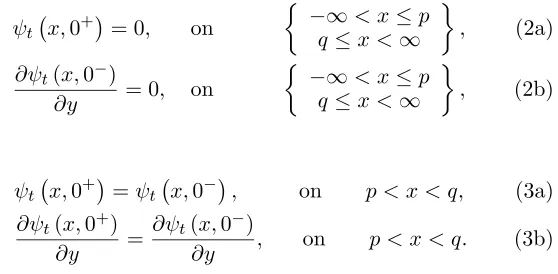
ψt
x,0+= 0, on
−∞< x≤p q ≤x <∞
, (2a)
∂ψt(x,0−)
∂y = 0, on
−∞< x≤p q ≤x <∞
, (2b)
and
ψt
x,0+=ψt
x,0−, on p < x < q, (3a)
∂ψt(x,0+)
∂y =
∂ψt(x,0−)
In Eqs. (2), (3), 0± refers to the situation thaty →0 through positive or negativey−axis.Let a plane acoustic wave
ψi=e−ik(xcosθ0+ysinθ0), (4)
be incident upon the slit occupying the position p≤x≤q, y = 0. I n Eq. (4),θ0 is the angle of incidence and for the analytic convenience it is assumed that the wave number k has positive imaginary part. For the analysis purpose it is convenient to express the total field ψt as
ψt=
ψi+ψr+ψ y >0
ψ y <0 , (5)
whereψ is the diffracted field andψr is the reflected field given by
ψr=−e−ik(xcosθ0+ysinθ0).
For the unique solution of the problem, the edge conditions require thatψt and its normal derivative must be bounded and satisfy [2].
ψt(x,0) =
−1 +O(x−p)14 as x→p−,
−1 +O(x−q)14 as x→q+,
(6)
∂ψt(x,0)
∂y =
O(x−p)−34 as x→p−, O(x−q)−34 as x→q+,
(7)
where a negative sign indicates a limit taken from left and a positive sign indicates that a limit taken from right. Thus, the scattered field satisfies the Helmholtz equation
∂2 ∂x2 +
∂2 ∂y2 +k
2
ψ(x, y) = 0, (8)
subject to the boundary conditions
ψx,0+= 0 on
−∞< x < p
q < x <∞ , (9a) and
∂ψ(x,0−)
∂y = 0 on
−∞< x < p
q < x <∞ , (9b) and the continuity conditions
and
∂ψ(x,0+) ∂y −
∂ψ(x,0−)
∂y = 2iksinθ0e
−ikxcosθ0 on p≤x≤q. (10b)
The Fourier transform pair is defined as follows
ψ(α, y) = 1 2π
∞
−∞
ψ(x, y)eiαxdx,
= eiαpψ−(α, y) +Q(α, y) +eiαqψ+(α, y), (11)
and its inverse as
ψ(x, y) = ∞
−∞
ψ(α, y)e−iαxdα, (12)
where
ψ−(α, y) = 1 2π
p
−∞
ψ(x, y)eiα(x−p)dx,
Q(α, y) = 1 2π
q
p
ψ(x, y)eiαxdx,
ψ+(α, y) = 1 2π
∞
q
ψ(x, y)eiα(x−q)dx. (13)
The function ψ−(α, y) is regular in the lower half plane Imα < Imk, ψ+(α, y) is regular in the upper half plane Imα >Imkcosθ0and Q(α, y) is an analytic function and therefore regular in the common region Imkcosθ0 <Imα <Imk.
On taking the Fourier transform of the Eq. (8) we arrive at
d2ψ(α, y) dy2 +K
2ψ(α, y) = 0, (14)
whereK(α) =√k2−α2.
from α=k toα=k∞ or from α=−k toα=−k∞. The solution of Eq. (14), representing the outgoing waves at infinity, can formally be written as
ψ(α, y) =
A(α)eiK(α)y y >0,
B(α)e−iK(α)y y <0, (15)
where A(α) and B(α) are the unknown coefficients which are to be determined. The Fourier transform of the boundary conditions (9) and (10) yields
ψ−1α,0+ = 0, (16a)
ψ+1α,0+ = 0, (16b)
ψ−2α,0− = 0, (16c)
ψ+2α,0− = 0, (16d)
Q1α,0+−Q1α,0− = 0, (17a) Q2
α,0+−Q2
α,0− = ksinθ0G(α), (17b)
where
ψ−1α,0− = 1 2π
p
−∞
ψx,0−eiα(x−p)dx, (18a)
ψ+1α,0− = 1 2π
∞
q
ψx,0−eiα(x−q)dx, (18b)
ψ−2α,0+ = 1 2πi
p
−∞
∂ψ(x,0+) ∂y e
iα(x−p)dx, (18c)
ψ+2α,0+ = 1 2πi
∞
q
∂ψ(x,0+) ∂y e
iα(x−q)dx, (18d)
Q1α,0+ = 1 2π
q
p
ψx,0+eiαxdx, (18e)
Q2α,0− = 1 2πi
q
p
∂ψ(x,0−) ∂y e
and
G(α) = e
i(α−kcosθ0)q−ei(α−kcosθ0)p
π(α−kcosθ0) . (19) Using Eqs. (16a)–(16d) and (17a)–(17b) in Eq. (15), we obtain
A(α)=Q1α,0+, (20a)
B(α)=−Q2
α,0−
K(α) , (20b)
A(α)−B(α)=−eiαpψ−1α,0−−eiαqψ+1α,0−, (20c)
−K(α) [A(α) +B(α)]=−eiαpψ−2α,0+−eiαqψ+2α,0++iksinθ0G(α). (20d)
The elimination of the coefficients A(α) and B(α) among the Eqs. (20a)–(20d) will lead to the following matrix Wiener-Hopf equation valid in the strip of analyticity Imkcosθ0 <Imα <Imk,
eiαq
ψ+1(α) ψ+2(α)
+
1 1
K(α)
−K(α) 1
Q1(α) Q2(α)
+eiαp
ψ−1(α) ψ−2(α)
=G(α)
0 iksinθ0
. (21)
In compact form, Eq. (21) can further be arranged as
eiαqΨ+(α) +H(α)Q(α) +eiαpΨ−(α) =G(α)A, (22) where bold letters are used to denote the matrices. Eq. (22) is an equation analogous to the Eq. (5.60) available in [31]. In Eq. (22),
H(α) is the kernel matrix and in order to solve it, we have to factorize the matrix H(α) as the product of two non-singular factor matrices such that one factor matrix being regular in the lower half plane and the other factor matrix being regular in the upper half plane with the additional requirements that both the factor matrices as well as their inverses contains elements of algebraic growth at infinity and both of these factor matrices should commute with each other. The factorization ofH(α), satisfying these conditions, has been done in [2] by using the Daniele-Kharapkov method [28, 29] and the result is as follows:
H+(α) = 2 1 4
coshχ(α) sinhχ(α)/γ(α) γ(α) sinhχ(α) coshχ(α)
, (23a)
with
H−(α) = H+(−α), (23b) where
χ(α) = −i 4arccos
α
k, χ(−α) =− i 4
π−arccosα k
and
γ(α) = α2−k2. (23d) Also as|α| → ∞, we note that
H±(α)∼(4k)−14
(±α)14 (±α)− 3 4
(±α)54 (±α) 1 4
. (23e)
After accomplishing the factorization of the matrix H(α), we can re-arrange Eq. (22) as
eiαqΨ+(α) +H+(α)H−(α)Q(α) +eiαpΨ−(α) =G(α)A. (24) Pre-multiplying Eq. (24) bye−iαq[H+(α)]−1, substituting the value of G(α) from Eq. (19) and simplifying we arrive at
[H+(α)]−1Ψ+(α) +e−iαqH−(α)Q(α) +eiα(p−q)[H+(α)]−1Ψ−(α) = e−
ikcosθ0q
π(α−kcosθ0)
[H+(α)]−1A−
eiα(p−q)−ikcosθ0p π(α−kcosθ0)
[H+(α)]−1A. (25) According to the procedure defined in [31] different terms occurring Eq. (25) can be decomposed as follows,
eiα(p−q)[H+(α)]−1Ψ−(α) = U+(α) +U−(α), (26) eiα(p−q)−ikcosθ0p
π(α−kcosθ0) [H+(α)]
−1A = V
+(α) +V−(α). (27) The pole contribution of the first term on right hand side of Eq. (25) can be expressed as
e−ikcosθ0q
π(α−kcosθ0)
{H+(α)}−1− {H+(kcosθ0)}−1+{H+(kcosθ0)}−1
A. (28) Using Eqs. (26)–(28) in Eq. (25) and separating it into positive and negative terms, we obtain
[H+(α)]−1Ψ+(α) +U+(α)
− e−ikcosθ0q
π(α−kcosθ0)
{H+(α)}−1− {H+(kcosθ0)}−1
A+V+(α) =−e−iαqH−(α)Q(α)−U−(α)−V−(α)+ e
−ikcosθ0q
π(α−kcosθ0){H+(kcosθ0)}
−1
where
U±(α) =± 1 2πi
∞+ic
−∞+ic
eiξ(p−q)[H
+(ξ)]−1Ψ−(ξ)
ξ−α dξ, (30) and
V±(α) =± 1 2πi
∞+ic
−∞+ic
eiξ(p−q)−ikcosθ0p[H
+(ξ)]−1A
π(ξ−α)(ξ−kcosθ0) dξ. (31) Now pre-multiplying Eq. (24)e−iαp[H−(α)]−1, substituting the value of G(α) from Eq. (19) and simplifying we arrive at
eiα(q−p)[H−(α)]−1Ψ+(α) +e−iαpH+(α)Q(α) + [H−(α)]−1Ψ−(α) =e
iα(q−p)−ikcosθ0q
π(α−kcosθ0)
[H−(α)]−1A− e−
ikcosθ0p
π(α−kcosθ0)
[H−(α)]−1A. (32) Decomposing different terms in Eq. (32) by following [31], we obtain
eiα(q−p)[H−(α)]−1Ψ+(α) = R+(α) +R−(α), (33) eiα(q−p)−ikcosθ0q
π(α−kcosθ0) [H−(α)]
−1A = S
+(α) +S−(α), (34) so that
R±(α) =± 1 2πi
∞+id
−∞+id
eiξ(q−p)[H−(ξ)]−1Ψ+(ξ)
ξ−α dξ, (35) and
S±(α) =± 1 2πi
∞+id
−∞+id
eiξ(q−p)−ikcosθ0q[H
−(ξ)]−1A π(ξ−α) (ξ−kcosθ0)
dξ, (36)
where −Imα < c < Imkcosθ0 and −Imα < d < Imkcosθ0, also Imα > c in Eqs. (30), (31) and Imα < d in Eqs. (35), (36) as given in [31].
Using Eqs. (33), (34) in Eq. (32) and separating it into positive and negative portions we arrive at
R−(α)+[H−(α)]−1Ψ−(α)−S−(α) + e−
ikcosθ0p
π(α−kcosθ0)
[H−(α)]−1A
The left hand side of Eq. (29) and right hand side of Eq. (37) are regular in Imα >Imkcosθ0 and right hand side of Eq. (29) and left hand side of Eq. (37) are regular in Imα <Imk. Hence using the extended form of the Liouville’s theorem each side of Eqs. (29) and (37) is equal to zero, i.e.,
[H+(α)]−1Ψ+(α) +U+(α)−
e−ikcosθ0q π(α−kcosθ0)
{H+(α)}−1− {H+(kcosθ0)}−1
A+V+(α) = 0, (38) and
R−(α) + [H−(α)]−1Ψ−(α)−S−(α) + e
−ikcosθ0p
π(α−kcosθ0)[H−(α)]
−1
A= 0. (39) Using Eqs. (30), (31) in Eq. (38) and Eqs. (35), (36) in Eq. (39) and simplifying these equations we obtain
[H+(α)]−1Ψ∗+(α) +
e−ikcosθ0q[H
+(kcosθ0)]−1A π(α−kcosθ0) + 1
2πi ∞+ic
−∞+ic
eiξ(p−q)[H+(ξ)]−1Ψ−(ξ)
(ξ−α) dξ= 0 (40)
and
[H−(α)]−1Ψ−(α)− 1 2πi
∞+id
−∞+id
eiξ(q−p)[H
−(ξ)]−1Ψ∗+(α)
(ξ−α) dξ= 0, (41) where
Ψ∗+(α) = Ψ+(α)−
e−ikcosθ0qA π(α−kcosθ0)
, (42)
Ψ−(α) = Ψ−(α) + e−
ikcosθ0pA
π(α−kcosθ0). (43) From the assumption that 0 < θ0 < π2, we can choose a such that
we arrive at
[H+(α)]−1Ψ∗+(α) +
e−ikcosθ0q[H
+(kcosθ0)]−1A π(α−kcosθ0)
− 1
2πi ∞+ia
−∞+ia
eiξ(q−p)[H−(ξ)]−1Ψ−(−ξ)
(ξ+α) dξ= 0 (44)
and
[H+(α)]−1Ψ−(−α)− 1 2πi
∞+ia
−∞+ia
eiξ(q−p)[H
−(ξ)]−1Ψ∗+(α)
(ξ+α) dξ= 0. (45)
Adding and subtracting Eqs. (44) and (45), we obtain
[H+(α)]−1S∗+(α) +
e−ikcosθ0q[H
+(kcosθ0)]−1A π(α−kcosθ0)
− 1
2πi ∞+ia
−∞+ia
eiξ(q−p)[H−(ξ)]−1S∗+(ξ)
(ξ+α) dξ= 0 (46)
and
[H+(α)]−1D∗+(α) +
e−ikcosθ0q[H
+(kcosθ0)]−1A π(α−kcosθ0) + 1
2πi ∞+ia
−∞+ia
eiξ(q−p)[H−(ξ)]−1D∗+(ξ)
(ξ+α) dξ= 0, (47)
where
S∗+(α) = Ψ∗+(α) + Ψ−(−α), (48)
D∗+(α) = Ψ∗+(α)−Ψ−(−α). (49) The Eqs. (46), (47) are of the same type and we obtain an approximate solution by a method due to Jones [32]. Setting
the Eqs. (46), (47) will take the form
[H+(α)]−1F∗+(α) + λ 2πi
∞+ia
−∞+ia
eiξ(q−p)[H−(ξ)]−1F∗+(ξ) (ξ+α) dξ
= −e
−ikcosθ0q[H
+(kcosθ0)]−1A
π(α−kcosθ0) , (51) where
F∗+(α) = F+(α)−
e−ikcosθ0qA π(α−kcosθ0)+
λe−ikcosθ0pA
π(α+kcosθ0), (52)
F+(α) = Ψ+(α)−λΨ−(−α), (53) and λ=±1.
A more elaborative form of Eq. (51) is as follows:
coshκ(α)F+1∗(α)−sinhκ(α)F+2∗(α)/γ(α)
−γ(α) sinhκ(α)F+1∗(α) + coshκ(α)F+2∗(α)
+ λ 2πi
∞+ia
−∞+ia
eiξ(q−p) (ξ+α)
coshκ(−ξ)F+1∗(ξ)−sinhκ(−ξ)F+2∗(ξ)/γ(−ξ)
−γ(−ξ) sinhκ(−ξ)F1∗
+ (ξ) + coshκ(−ξ)F+2∗(ξ)
dξ
+ e
−ikcosθ0q
π(α−kcosθ0)
A1coshκ(kcosθ0)−A2sinhκ(kcosθ0)/γ(kcosθ0)
−A1γ(kcosθ0) sinhκ(kcosθ0) +A2coshκ(kcosθ0)
= 0. (54)
Eq. (52) in matrix form can be written as:
F+1∗(α) F+2∗(α)
= F1 +(α) F1 +(α)
− e−ikcosθ0q
π(α−kcosθ0)
A1 A2
+ λe
−ikcosθ0p
π(α+kcosθ0)
A1 A2
. (55)
Considering the first row of Eq. (54) and using the values of F+1∗(α) and F+2∗(α) in it, we obtain
coshκ(α)
F+1(α)− e−
ikcosθ0q
π(α−kcosθ0) A1+
λe−ikcosθ0p π(α+kcosθ0)
A1
−sinhκ(α)
γ(α)
F+2(α)− e
−ikcosθ0q
π(α−kcosθ0) A2+
λe−ikcosθ0p π(α+kcosθ0)
A2
∞+ia
−∞+ia
eiξ(q−p) (ξ+α)
coshκ(−ξ)
F+1(ξ)− e−
ikcosθ0q
π(ξ−kcosθ0) A1+
λe−ikcosθ0p π(ξ+kcosθ0)
A1
−sinhκ(−ξ)/γ(ξ)
F+2(ξ)− e
−ikcosθ0q
π(ξ−kcosθ0) A2+
λe−ikcosθ0p π(ξ+kcosθ0)
A2
dξ
+ e
−ikcosθ0q
π(α−kcosθ0)
[A1coshκ(kcosθ0)−A2sinhκ(kcosθ0)/γ(kcosθ0)]
= 0. (56)
Writingγ(ξ) =γ+(ξ)γ−(ξ) =
√
ξ+k√ξ−k and considering the integrals arising in Eq. (56), we have
I = I1−
e−ikcosθ0qA 1 π I2+
λe−ikcosθ0pA 1 π I3−I4 +e
−ikcosθ0qA2
π I5+
e−ikcosθ0pA2
π I6, (57)
where
I1 = ∞+ia
−∞+ia
eiξ(q−p)coshκ(−ξ)F+1(ξ)
(ξ+α) dξ, (58)
I2 = ∞+ia
−∞+ia
eiξ(q−p)coshκ(−ξ) (ξ+α) (ξ−kcosθ0)
dξ, (59)
I3 = ∞+ia
−∞+ia
eiξ(q−p)coshκ(−ξ)
(ξ+α) (ξ+kcosθ0)dξ, (60)
I4 = ∞+ia
−∞+ia
eiξ(q−p)F+2(ξ) sinhκ(−ξ)/√ξ+k
(ξ+α)√ξ−k dξ, (61)
I5 = ∞+ia
−∞+ia
eiξ(q−p)sinhκ(−ξ)/√ξ+k
(ξ−kcosθ0) (ξ+α)√ξ−kdξ, (62)
I6 = ∞+ia
−∞+ia
eiξ(q−p)sinhκ(−ξ)/√ξ+k (ξ+kcosθ0) (ξ+α)
√
Integrals (58)–(63) are solved by a method described in [31] and are substituted in Eq. (56) to get
coshκ(α)
F+1(α)− e
−ikcosθ0q
π(α−kcosθ0)
A1+ λe
−ikcosθ0p
π(α+kcosθ0) A1
−sinhκ(α)
γ(α)
F+2(α)− e
−ikcosθ0q
π(α−kcosθ0)
A2+ λe
−ikcosθ0p
π(α+kcosθ0) A2
=
−λT(α)F+1(k) +λe
−ikcosθ0q
π
×A1
eiklcosθ0 (α+kcosθ0)
coshκ(−kcosθ0) +R2(α)
−A1e
−ikcosθ0p
π R1(α) +λT1(α)F 2
+(k)−λ
e−ikcosθ0q π A2
×
eiklcosθ0sinhκ(−kcosθ
0)/γ+(kcosθ0)
(α+kcosθ0)γ−(kcosθ0) +R4(α)
−A2
e−ikcosθ0p
π R3(α)−
e−ikcosθ0q π(α−kcosθ0)
×[A1coshκ(kcosθ0)−A2sinhκ(kcosθ0)/γ(kcosθ0)], (64) wherel=q−p and
T(α) = 1
2πiE−12W− 1
2{−i(k+α)l}, T1(α) = 1
2πiE−1W−1{−i(k+α)l}, R1,2(α) =
coshκ(−k)E−1 2
W−1
2{−i(k±kcosθ0)l} −W− 1
2{−i(k+α)l}
2πi(α∓kcosθ0) ,
R3,4(α) =
E−1[W−1{−i(k±kcosθ0)l} −W−1{−i(k+α)l}] sinhκ(−k)/
√
2k 2πi(α∓kcosθ0)
.
(65)
described in [31] and the result is
coshκ(α)F+1(α)−sinhκ(α) γ(α) F
2 +(α)
= −λT(α)F+1(k) +λT1(α)F+2(k) +A1e
−ikcosθ0q
π P1(α)
−λA1
e−ikcosθ0p
π P2(α)−A2
e−ikcosθ0q
π P3(α) +λA2
e−ikcosθ0p π P4(α)
+λA1e
−ikcosθ0q
π R2(α)−A1
e−ikcosθ0p
π R1(α)−λA2
e−ikcosθ0q π R4(α)
+A2
e−ikcosθ0p
π R3(α), (66)
where
P1(α) =
1 (α−kcosθ0)
[coshκ(α)−coshκ(kcosθ0)], P2(α) =
1 (α+kcosθ0)
[coshκ(α)−coshκ(−kcosθ0)], P3(α) =
1 (α−kcosθ0)
sinhκ(α) γ(α) −
sinhκ(kcosθ0) γ(kcosθ0)
,
P4(α) =
1
γ−(−kcosθ0)(α+kcosθ0)
sinhκ(α) γ(α) −
sinhκ(−kcosθ0) γ+(kcosθ0)
.
(67)
Further simplification of Eq. (66) will yield
coshκ(α)F+1(α)−sinhκ(α) γ(α) F
2 +(α)
= −λT(α)F+1(k) coshκ(−k) +λT1(α)F+2(k)sinh√κ(−k) 2k
+A1 π {e
−ikcosθ0qP
1(α)−e−ikcosθ0pR1(α)}
−λA1
π {e
−ikcosθ0pP2(α)−e−ikcosθ0qR2(α)}
−A2 π {e
−ikcosθ0qP
3(α)−e−ikcosθ0pR3(α)} +λA2
π {e
Letting
G1(α) = e−ikcosθ0qP1(α)−e−ikcosθ0pR1(α), G2(α) = e−ikcosθ0pP2(α)−e−ikcosθ0qR2(α), G3(α) = e−ikcosθ0qP3(α)−e−ikcosθ0pR3(α),
G4(α) = e−ikcosθ0pP4(α)−e−ikcosθ0qR4(α), (69) in Eq. (68), the solution of the first WH equation, obtained by considering the first row of matrices in Eq. (54), is given as follows:
coshκ(α)F+1(α)− sinhκ(α)F 2 +(α)
γ(α) =−λT(α) coshκ(−k)F 1 +(k)
+λT1(α) sinhκ(−k)F 2 +(k)
√
2k +
A1
π [G1(α)−λG2(α)]
−A2
π [G3(α)−λG4(α)]. (70) The second WH equation corresponds to the second row of the matrix Eq. (54) and its solution can be obtained in a similar manner as for the first row of Eq. (54). Omitting all the similar steps and quantities arose in the solution, we finally arrive at:
−γ(α) sinhκ(α)F+1(α)+coshκ(α)F+2(α) =λT2(α)√2ksinhκ(−k)F+1(k)
−λT(α) coshκ(−k)F+2(k)+A2
π [G1(α)−λG2(α)]− A1
π [G5(α)−λG6(α)], (71)
where
T2(α) = 1
2πiE0W0{−i(k+α)l}
G5(α) = e−ikcosθ0qP5(α)−e−ikcosθ0pR5(α), G6(α) = e−ikcosθ0pP6(α)−e−ikcosθ0qR6(α),
P5(α) = γ(α) sinhκ(α)−γ(kcosθ0) sinhκ(kcosθ0) α−kcosθ0
,
P6(α) = γ(α) sinhκ(α)−γ(−kcosθ0) sinhκ(−kcosθ0) α+kcosθ0
,
R5,6(α) =
D0[W0{−i(k±kcosθ0)l} −W0{−i(k+α)l}] 2πi(α∓kcosθ0)
,
D0 = E0
√
In Eqs. (65) and (72), we have
Wn−1 2 (z) =
∞
0 une−u
u+zdu
= Γ (n+ 1)e12zz 1 2n−
1 2W
−1 2(n+1),
1
2n(z), (73)
wherez=−i(k+α)landn=−12,0,12. Wm,nis known as a Whittaker
function [32]. The values of the functions F+1(k) and F+2(k) can be calculated by putting α =k in Eqs. (70) and (71) and solving these equations simultaneously. Now as
F+(α) =
F+1(α) F+2(α)
=
ψ+1(α)
ψ+2(α)
−λ
ψ−1(α)
ψ−2(α)
, (74)
Eq. (74) is considered for the cases λ= 1 and λ=−1 and when the values of F1
+(α) and F+2(α) are substituted in Eqs. (70) and (71) the results are as follows:
Forλ= 1
coshκ(α)ψ+1(α)−ψ−1(α)−sinhκ(α) γ(α)
ψ+2(α)−ψ−2(α) = −T(α) coshκ(−k)F+1(k)λ=1+T1(α) sinh√ κ(−k)
2k F
2
+(k)λ=1
+A1
π [G1(α)−G2(α)]− A2
π [G3(α)−G4(α)], (75) and
−γ(α) sinhκ(α)ψ+1(α)−ψ−1(α)+ coshκ(α)ψ+2(α)−ψ−2(α) =−T(α) coshκ(−k)F+2(k)λ=1+√2kT2(α) sinhκ(−k)F+1(k)λ=1 +A2
π [G1(α)−G2(α)]− A1
π [G5(α)−G6(α)], (76) and for λ=−1
coshκ(α)ψ+1(α) +ψ−1(α)−sinhκ(α) γ(α)
ψ+2(α) +ψ−2(α)
= +T(α) coshκ(−k)F+1(k)λ=−1−T1(α) sinh√ κ(−k)
2k F
2
+(k)λ=−1
+A1
π [G1(α) +G2(α)]− A2
and
−γ(α) sinhκ(α)ψ+1(α)+ψ−1(α)+coshκ(α)ψ+2(α)+ψ−2(α) = T(α) coshκ(−k)F+2(k)λ=−1−T2(α)√2ksinhκ(−k)F+1(k)λ=−1
+A2
π [G1(α) +G2(α)]− A1
π [G5(α) +G6(α)]. (78)
Adding Eqs. (75) and (77), we obtain
coshκ(α)ψ+1(α)−sinhκ(α)
γ(α) ψ+2(α)
= A1
π G1(α)− A2
π G3(α)−
T(α) coshκ(−k)
2 C1+
T1(α) sinhκ(−k) 2√2k C2,
(79)
and Eqs. (76) and (18) will yield
−γ(α) sinhκ(α)ψ+1(α)+coshκ(α)ψ+2(α) = A2
π G1(α)− A1
π G5(α)−
T(α) coshκ(−k)
2 C2
+T2(α)
√
2ksinhκ(−k)
2 C1. (80)
where
C1 = F+1(k)λ=1−F+1(k)λ=−1,
C2 = F+2(k)λ=1−F+2(k)λ=−1. (81) Eliminatingψ+2(α) from Eqs. (79) and (80), we obtain
ψ+1(α) =
A1
π coshκ(α)+ A2
π
sinhκ(α) γ(α)
G1(α)−A2
π G3(α) coshκ(α)
−A1 π G5(α)
sinhκ(α) γ(α) −
T(α) coshκ(−k) 2
C1coshκ(α)+C2
sinhκ(α) γ(α)
+T1(α) sinhκ(−k) coshκ(α)C2 2√2k
+T2(α)
√
2ksinhκ(−k) sinhκ(α)/γ(α)C1
and eliminatingψ+1(α) between Eqs. (79) and (80), will yield
ψ+2(α) =
A1
π γ(α) sinhκ(α) + A2
π coshκ(α)
G1(α)
−A2
π G3(α)γ(α) sinhκ(α)− A1
π G5(α) coshκ(α)
−T(α) coshκ(−k)
2 (C1γ(α) sinhκ(α) +C2coshκ(α))
+T1(α) sinhκ(−k)γ(α) sinhκ(α)C2 2√2k
+T2(α)
√
2ksinhκ(−k) coshκ(α)C1
2 . (83)
Now in order to calculate the function ψ−1(α) andψ−2(α) we replace G1(α) byG2(α) (andG2(α) byG1(α)),G3(α) byG4(α) (andG4(α) by G3(α)) andG5(α) byG6(α) (andG6(α) byG5(α)) and also changing α to−α in the Eqs. (82)and (83), respectively, we arrive at:
ψ−1(α) =
A1
π coshκ(−α) + A2
π
sinhκ(−α) γ(−α)
G2(−α)
−A2
π G4(−α) coshκ(−α)− A1
π G6(−α)
sinhκ(−α) γ(−α)
−T(−α) coshκ(−k)
2
C1coshκ(−α) +C2
sinhκ(−α) γ(−α)
+T1(−α) sinhκ(−k) coshκ(−α)C2 2√2k
+T2(−α)
√
2ksinhκ(−k) sinhκ(−α)/γ(−α)C1
2 , (84)
and
ψ−2(α) =
A1
π γ(−α) sinhκ(−α) + A2
π coshκ(−α)
G2(−α)
−A2
π G4(−α)γ(−α) sinhκ(−α)− A1
π G6(−α) coshκ(−α)
−T(−α) coshκ(−k)
2
C1γ(−α) sinhκ(−α)+C2coshκ(−α)
+T1(−α) sinhκ(−k)γ(−α) sinhκ(−α)C2 2√2k
+T2(−α)
√
2ksinhκ(−k) coshκ(−α)C1
whereC1 and C2 are given by
C1 = F+1(k)
λ=1−
F+1(k)
λ=−1,
C2 = F+2(k)
λ=1−
F+2(k)
λ=−1, (86)
and F+1(k) and F+2 (k) denote the functions in which G1 by G2 and G2 by G1, G3 by G4 and G4 by G3 and G5 by G6 and G6 by G5 have also been interchanged and then evaluated for λ = 1 and λ = −1 respectively. Since the functions ψ±1(α) and ψ±2(α) have been calculated, therefore we now manipulate Eqs. (20c) and (20d) and the unknown coefficientA(α) is determined to be
A(α) = 1 2K(α)
eiαpψ−2(α)−iksinθ0G(α) +eiαqψ+2(α)
−eiαpψ−1(α)
2 −
eiαqψ+1(α)
2 . (87)
Substituting the values of ψ±1(α) and ψ±2(α) in Eq. (87) and simplifying we obtain
A(α) =
1 2πK(α)
iksinθ0coshκ(−α) coshκ(−kcosθ0) α−kcosθ0 e
i(α−kcosθ0)p
−iksinθ0R2(−α) coshκ(−α)eiαp−kcosθ0q
−iksinθ0sinhκ(−α)γ(−α) sinhκ(−kcosθ0)
(α−kcosθ0)γ(−kcosθ0) e
i(α−kcosθ0)p
+iksinθ0R4(−α)γ(−α) sinhκ(−α)eiαp−kcosθ0q +
T(−α) coshκ(−k) 2
−γ(−α) sinhκ(−α)C1 + coshκ(−α)C2
+T1(−α)γ(−α) sinhκ(−α) sinhκ(−k)C2 2√2k
+T2(−α) sinhκ(−k) coshκ(−α)
√
2kC1 2
eiαp
+ 1
2πK(α)
−iksinθ0coshκ(α) coshκ(kcosθ0) α−kcosθ0 e
i(α−kcosθ0)q
−iksinθ0R1(α) coshκ(α)eiαq−ikcosθ0p +iksinθ0sinhκ(α)γ(α) sinhκ(kcosθ0)
(α−kcosθ0)γ(kcosθ0)
+iksinθ0R3(α)γ(α) sinhκ(α)eiαq−kcosθ0pq
+
T(α) coshκ(−k)
2 (−γ(α) sinhκ(α)C1−coshκ(α)C2) +T1(α)γ(α) sinhκ(α) sinhκ(−k)C2
2√2k +T2(α) sinhκ(−k) coshκ(α)
√
2kC1 2
eiαq
+ 1 2π
−iksinθ0sinhκ(−α) coshκ(−kcosθ0) γ(−α) (α−kcosθ0)
ei(α−kcosθ0)p
+iksinθ0coshκ(−α) sinhκ(−kcosθ0) (α−kcosθ0)γ(−kcosθ0)
ei(α−kcosθ0)p
+iksinθ0R2(−α)sinhκ(−α)e
iαp−kcosθ0q
γ(−α)
−iksinθ0R4(−α)coshκ(−α)eiαp−kcosθ0q +
−T(−α) coshκ(−k) 2
coshκ(−α)C1+
sinhκ(−α) γ(−α) C2
+T1(−α) sinhκ(−k) coshκ(−α)C2 2√2k
+ T2(−α) sinhκ(−k) sinhκ(−α)
√
2kC1 2
eiαp
+ 1 2π
iksinθ0sinhκ(α) coshκ(kcosθ0) γ(α) (α−kcosθ0)
ei(α−kcosθ0)q
−iksinθ0coshκ(α) sinhκ(kcosθ0)
(α−kcosθ0)γ(−kcosθ0)
ei(α−kcosθ0)q
−iksinθ0R3(α) coshκ(α)eiαq−kcosθ0p +iksinθ0R1(α) sinhκ(α)e
iαq−kcosθ0p
γ(α)
−
−T(−α) coshκ(−k) 2
coshκ(α)C1+sinhκ(α) γ(α) C2
+T1(α) sinhκ(−k) coshκ(α)C2 2√2k
+ T2(α) sinhκ(−k) sinhκ(α)
√
2kC1 2γ(α)
eiαq
Since A(α) has been determined, the scattered field ψ(x, y) can now be determined by substituting A(α) into Eq. (15) and taking the inverse Fourier transform, we shall arrive at
ψ(x, y) = ∞
−∞
A(α)eiK(α)y−iαxdα, (89)
where A(α) is defined in Eq. (88). The scattered fieldψ(x, y) can be split up into two components as follows:
ψ(x, y) =ψsep(x, y) +ψint(x, y), (90)
where
ψsep(x, y) =
∞
−∞
1
2πK(α)
iksinθ0coshκ(−α) coshκ(−kcosθ0)
−iksinθ0sinhκ(−α)γ(−α) sinhκ(−kcosθ0) γ(−kcosθ0)
+ 1 2π
−iksinθ0sinhκ(−α) coshκ(−kcosθ0) γ(−α)
+iksinθ0coshκ(−α) sinhκ(−kcosθ0) γ(−kcosθ0)
ei(α−kcosθ0)p α−kcosθ0
+ 1
2πK(α){(−iksinθ0coshκ(α) coshκ(kcosθ0) +iksinθ0sinhκ(α)γ(α) sinhκ(kcosθ0)
γ(kcosθ0)
+ 1 2π
iksinθ0sinhκ(α) coshκ(kcosθ0) γ(α)
−iksinθ0coshκ(α) sinhκ(kcosθ0) γ(kcosθ0)
ei(α−kcosθ0)q α−kcosθ0
eiK(α)y−iαxdα,
(91)
and
ψint(x, y) =
∞
−∞ 1
2πK(α)[{(−iksinθ0coshκ(α)R1(α) +iksinθ0sinhκ(α)γ(α)R3(α))eiαq−ikcosθ0p
+
T(α) coshκ(−k)
+T1(α)γ(α) sinhκ(α) sinhκ(−k)C2 2√2k
+ T2(α)
√
2ksinhκ(−k) coshκ(α)C1 2
eiαq
+ 1
2πK(α){(−iksinθ0coshκ(−α)R2(−α)
+iksinθ0sinhκ(−α)γ(−α)R4(−α))eiαp−ikcosθ0q +
T(−α) coshκ(−k) 2
−γ(−α) sinhκ(−α)C1−coshκ(−α)C2
+T1(−α)γ(−α) sinhκ(−α) sinhκ(−k)C2 2√2k
+T2(−α)
√
2ksinhκ(−k) coshκ(−α)C1 2
eiαp
+ 1 2π
−iksinθ0coshκ(α)R3(α) +iksinθ0
sinhκ(α) γ(α) R1(α)
×eiαq−ikcosθ0p−
−T(α) coshκ(−k) 2
C1coshκ(α) +C2
sinhκ(α) γ(α)
+T1(α) sinhκ(−k) coshκ(α)C2 2√2k
+ T2(α)
√
2ksinhκ(α) sinhκ(−k)C1 2
eiαq
+ 1 2π
iksinθ0sinhκ(−α)R2(−α)
γ(−α) −iksinθ0coshκ(−α)R4(−α)
×eiαp−ikcosθ0q
−
T(−α) coshκ(−k) 2
−C1 coshκ(−α)−C2 sinhκ(−α) γ(−α)
+T1(−α) sinhκ(−k) coshκ(−α)C2 2√2k
+T2(α)
√
2ksinhκ(−α) sinhκ(−k)C1 2
eiαp
eiK(α)y−iαxdα, (92)
where ψsep(x, y) gives the diffracted field produced by the edges at
x=p and atx=q respectively andψint(x, y) gives the interaction of
θ
Figure 2. Variation of the separated fieldψsepwith observation angle
θatθ0 = π4,k= 1 and l= 1.
2.1. Far-Field Solution
The calculations carried out for the three part boundary value problem formulated in terms of matrix WH equations are quite laborious and delicate at the same time, so we report the far field only for the case of y > 0 only, (i.e., we determine the unknown coefficient A(α) only), the far field for the case of y < 0 can be calculated in a similar manner. Therefore, in order to solve the integral appearing in Eq. (89) we introduced the following substitutions
x=ρcosθ, y=ρsinθ and α=−kcos (θ+it1), (93) in Eq. (89), omitting the computational details, and using the method of steepest descent, the field at the large distance from a slit in an infinite soft-hard plane is given as
ψ(x, y)
"
2π
kρisinθA(−kcosθ)e
ikρ+iπ4. (94)
whereA(−kcosθ) can be evaluated from Eq. (88).
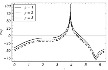
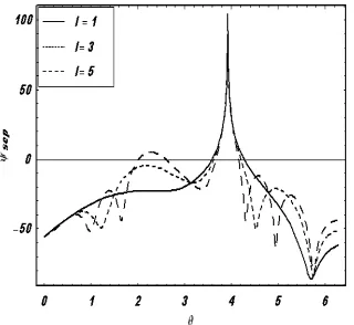
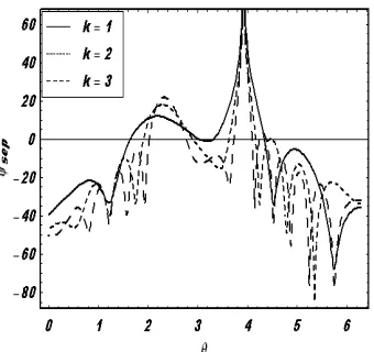
3. GRAPHICAL RESULTS
In this section we will present some graphs showing the effects of various parameters on the diffracted field produced by the two edges of the slit in an infinite soft-hard plane.
Figs. 2 and 3 show the variation of separated field ψsep with
θ
Figure 3. Variation of the separated fieldψsepwith observation angle
θatθ0 = π4,k= 1 and l= 5.
Figure 4. Variation of the separated fieldψsepwith observation angle
θatθ0 = π4, ρ= 1 and k= 1.
Figure 5. Variation of the separated fieldψsepwith observation angle
Figure 6. Variation of the separated fieldψsepwith observation angle
θatθ0 = π4, ρ= 1 and l= 1.
Figure 7. Variation of the separated fieldψsepwith observation angle
θatθ0 = π4, ρ= 1 and l= 5.
4. CONCLUSION
In this paper the diffraction of a plane acoustic wave by a slit in an infinite soft hard plane is investigated rigorously with the help of integral transform, Wiener-Hopf technique and the method of steepest descent. Further the consideration of slit in an infinite soft-hard plane will help understand acoustic diffraction and will go a step further to complete the discussion for the soft-hard half plane. The two edges of the slit give rise to two diffracted fields (one from each edge) and the interaction of one edge upon the other edge. The diffracted field is presented for the far-field situation and some graphs showing the effects of various parameters on the separated field are also plotted.
REFERENCES
1. Rawlins, A. D., “The solution of a mixed boundary value problem in the theory of diffraction by a semi-infinite plane,” Proc. Roy. Soc. London, Ser. A, Vol. 346, 469–484, 1975.
2. B¨uy¨ukaksoy, A., “A note on the plane wave diffraction by a soft/hard half-plane,”ZAMM, Vol. 75, No. 2, 162–164, 1995. 3. Hamid, M. A. K., A. Mohsen, and W. M. Boerner, “Diffraction
by a slit in a thick conducting screen,” J. Appl. Physics Communications, 3882–3883, 1969.
4. Keller, J. B., “Diffraction by an aperture,” J. Appl. Physics, Vol. 28, No. 4, 426–444, 1957.
5. Karp, S. N. and A. Russek, “Diffraction by a wide slit,” J. Appl. Physics, Vol. 27, No. 8, 886–894, 1956.
6. Levine, H., “Diffraction by an infinite slit,” J. Appl. Physics, Vol. 30, No. 11, 1673–1682, 1959.
7. Birbir, F. and A. B¨uy¨ukaksoy, “Plane wave diffraction by a wide slit in a thick impedance screen,” Journal of Electromagnetic Waves and Applications, Vol. 10, No. 6, 803–826, 1996.
8. Morse, P. M. and P. J. Rubenstein, “The diffraction of waves by ribbons and slits,”Phys. Rev., Vol. 54, 895–898, 1938.
9. Asghar, S., T. Hayat, and J. G. Haris, “Diffraction by a slit in an infinite porous barrier,”Wave Motion, Vol. 33, 25–40, 2001. 10. Hayat, T., S. Asghar, and K. Hutter, “Scattering from a slit in a
biisotropic medium,”Can. J. Phys., Vol. 81, 1193–1204, 2003. 11. Ahmed, S. and Q. A. Naqvi, “Electromagnetic scattering from a
12. Ayub, M., M. Ramzan, and A. B. Mann, “A note on spherical electromagnetic wave diffraction by a perfectly conducting strip in a homogeneous bi-isotropic medium,” Progress In Electromagnetics Research, PIER 85, 169–194, 2008.
13. Ghazi, G. and M. Shahabadi, “Modal analysis of extraordinary transmission through an array of subwavelength slits,” Progress In Electromagnetics Research, PIER 79, 59–74, 2008.
14. Imran, A., Q. A. Naqvi, and K. Hongo, “Diffraction of plane waves by two parallel slits in an infinitely long impedance plane using the method of Kobayashi potentials,” Progress In Electromagnetics Research, PIER, 63, 107–123, 2006.
15. Naveed, M. and Q. A. Naqvi, “Diffraction of EM plane wave by a slit in an impedance plane using Maliuzhinetz function,”Progress In Electromagnetics Research B, Vol. 5, 265–273, 2008.
16. Ayub, M., A. B. Mann, and M. Ahmad, “Line source and point source scattering of acoustic waves by the junction of transmissive and soft-hard half planes,”J. Math. Anal. Appl., Vol. 346, No. 1, 280–295, 2008.
17. Senior, T. B. A. and E. Topaskal, “Diffraction by an anisotropic impedance half plane-reviewed solution,”Progress In Electromagnetics Research, PIER 53, 1–19, 2005.
18. Liang, C. H., Z. Liu, and H. Di, “Study on the blockage of electromagnetic rays analytically,” Progress In Electromagnetics Research B, Vol. 1, 253–268, 2008.
19. Ghaffar, A., Q. A. Naqvi, and K. Hongo, “Analysis of the fields in three dimensional Cassegrain system,” Progress In Electromagnetics Research, PIER 75, 215–240, 2007.
20. Ghaffar, A., A. Hussain, and Q. A. Naqvi, “Radiation characteris-tics of an inhomogeneous slab,”Journal of Electromagnetic Waves and Applications, Vol. 22, No. 2, 301–312, 2008.
21. Ghaffar, A., Q. A. Naqvi, and K. Hongo, “Focal region fields of three dimensional Gregorian system,”Optics Communications, Vol. 281, 1343–1353, 2008.
22. Ghaffar A. and Q. A. Naqvi, “Focusing of electromagnetic plane wave into uniaxial crystal by a three dimensional plano-convex lense,” Progress In Electromagnetics Research, PIER 83, 25–24, 2007.
24. Ahmed S. and Q. A. Naqvi, “Electromagnetic scattering from paralell perfect electromagnetic conductor cylinders of circular cross-section using iterative procedure,” Journal of Electromagnetic Waves and Applications, Vol. 22, 987–1003, 2008. 25. Hurd, R. A., “A note on the solvability of simultaneous
Wiener-Hopf equations,”Can. J. Phys., Vol. 57, 402–403, 1979.
26. Rawlins, A. D., “The solution of mixed boundary value problem in the theory of diffraction,”J. Engng. Mathematics, Vol. 18, 37–62, 1984.
27. Rawlins, A. D. and W. E. Williams, “Matrix Wiener-Hopf factorization,” Quart. J. Mech. Appl. Math., Vol. 34, 1–8, 1981. 28. Daniele, V. G., “On the factorization of Wiener-Hopf matrices
in problems solvable with Hurd’s method,” IEEE Trans. on Antennas Propagat., Vol. 26, 614–616, 1978.
29. Kharapkov, A. A., “Certain cases of the elastic equilibrium of an infinite wedge with a non-symmetric notch at the vortex, subjected to concentrated forces,” Prikl. Math. Mekh., Vol. 35, 1879–1885, 1971.
30. B¨uy¨ukaksoy, A. and A. H. Serbest, “Matrix Wiener-Hopf factor-ization methods and applications to some diffraction problems,” Analytical and Numerical Techniques in Electromagnetic Wave Theory, Chap. 6., Hashimoto, Idemen, Tretyakov (eds.), Science House, Tokyo, Japan.
31. Noble, B., Methods Based on the Wiener-Hopf Technique, Pergamon, London, 1958.